Optimizing Vehicle Collision Safety: A Two-Mass Model with Dual Springs and Dampers for Accurate Crash Dynamics Prediction
Abstract:
A comprehensive analysis of vehicle collision dynamics is presented using a two-mass model that simulates the impact of a vehicle against a rigid barrier. The model incorporates dual springs and dampers to examine the influence of spring stiffness and damping on a mass attached to the vehicle. The equations of motion are solved utilizing state variables, while energy principles are employed to establish correlations between vehicle deformation, impact force, and acceleration. Validation is conducted through comparison with crash test data from a 2023 Honda Accord LX 4-Door Sedan. Average deformation values are used to calculate acceleration, followed by a Monte Carlo simulation to analyze acceleration data recorded by the engine sensor, enabling the determination of vehicle speed through integration. Parametric regression is applied to optimize model parameters, resulting in a high degree of concordance between experimental and theoretical values. The model's accuracy is further verified through the analysis of velocity and deceleration profiles and the integration of the deceleration curve. The findings underscore the model's capability to replicate real-world crash dynamics, highlighting its potential to enhance vehicle safety system design. The innovation of this research lies in its simplified yet effective approach to modeling collision dynamics, offering significant insights into the relationship between vehicle deformation and occupant forces. This work advances the understanding of vehicle collision mechanics and provides a robust tool for the development of advanced safety features. The integration of theoretical and empirical data reinforces the model's reliability, contributing substantively to the field of automotive safety engineering.
1. Introduction
Road traffic accidents are a major cause of serious injuries and fatalities globally, with over one million deaths and injuries reported annually by the World Health Organization (WHO) [1].
Since the 1970s and up to the present day, a great deal of research has focused on modeling road accidents in order to understand the collision mechanism and reduce their severity. Campbell developed a semi-empirical formula for estimating impact energy based on deformations [2]. Analysis indicates that specific height parameters of the rear, front, middle, and middle-backward parts of the system significantly impact occupant injury, OLC, and barrier bottoming out. Additionally, a study reveals that a concave-shaped crash pulse can enhance crashworthiness and compatibility. Another investigation explores the impact of structural downsizing on optimal structural crashworthiness in lightweight vehicles. It suggests that incorporating a sufficiently high relative deformable length and mean engine-to-body mass ratio can substantially improve crashworthiness, even in downsizing scenarios. The overall vehicle mass has a less significant effect on structural crashworthiness in barrier impacts. The best optimal crashworthiness performance within the studied range of vehicle sizes is achieved under specific design conditions [3]. Ludong Sun's study introduces a dynamic model for automotive side impact crashes, employing a low-order lumped parameter model (LPM) with high nonlinearity. Validation using National Highway Traffic Safety Administration (NHTSA) crash test data confirms the model's accuracy, showing applications for developing active occupant protection systems [4]. Koji Mizuno's research focuses on optimizing vehicle crash pulses to reduce injury risks for rear-seat occupants in frontal impacts. The optimized crash pulse, characterized by a concave shape, minimizes occupant deceleration and reduces chest acceleration and rib fracture risks, emphasizing its potential for enhancing vehicle safety [5].
A detailed analysis of vehicle suspension systems demonstrates how they manage dynamic loads during travel and impact scenarios. Suspension systems, whether passive, semi-active, or active, significantly affect vehicle stability and occupant comfort. Understanding the dynamic responses of these systems, particularly through modal analysis and finite element methods (FEM), aids in designing suspensions that can better manage the stresses of a crash [6]. Also, research on variable stiffness and damping control strategies highlights advancements in suspension technology, such as magnetorheological shock absorbers that adapt their responses based on driving conditions. These technologies offer potential for enhancing vehicle safety by actively modifying suspension characteristics in response to crash impacts, providing better protection and stability [7].
Another study aimed to improve Campbell's equation by finding a relationship between the two stiffness coefficients A and B on the basis of statistical findings and thus making the formula easier to use [8].
The mass-spring-Damper model is commonly employed to simulate vehicle collisions, providing a representation of the damping effect on the system [9]. [10], [11]. A study proposes a real-time, capable approach with two parallel paths to address this challenge: Path A uses a machine learning component trained with FEM data to predict crash severity in less than a millisecond. Path B employs a 2D mass-spring-damper model to estimate crash forces and accelerations, serving as a fallback and validation layer. Together, these paths provide accurate and reliable real-time predictions for collision scenarios [12]. In other studies, two types of LPMs are introduced to study vehicle frontal crashes. A four-degree-of-freedom (DOF) LPM hybrid (LH) model is proposed and compared with a serial 4-DOF model. Additionally, a 5-DOF LH model is proposed and compared with a serial 5-DOF model. Spring and damper coefficients are determined to match the deceleration of the models with experimental data, using a genetic algorithm (GA) for system identification to optimize these parameters. The study also examines absolute decelerations and their frequencies due to external load excitation [13].
State-of-the-art crash-worthiness techniques use simulations and physical tests. This paper proposes creating analytical models from crash test data using system identification techniques. The models combine differential equations and a transfer function (ARMA of white noise) with time-varying parameters estimated recursively. The method is validated with noise and applied to impact data, noting limitations and future work [14].
A paper presents a novel assessment method using a Bayesian probabilistic framework and real-time vibration data to identify collision damage and uncertainties. By integrating the Monte Carlo algorithm, the approach estimates the probability and extent of damage [15].
A paper presents a risk assessment procedure for vehicle crosswind stability, combining a random gust model with constrained simulations and variance-reducing Monte Carlo methods to efficiently compute failure probabilities. The procedure allows for investigating the impact of factors like turbulence, track irregularities, and wheel-road friction on stability [16].
In this paper, we introduce a comprehensive modeling and simulation approach to investigate vehicle collisions, taking into account the dynamic characteristics of vehicles, including mass, velocity, damping coefficients, and spring stiffness. Furthermore, we conducted an analysis and comparison of acceleration sensor records from frontal impacts on a 2023 Honda Accord LX 4-Door Sedan, sourced from the NHTSA database [17]. The aim is to extract pertinent information regarding the variations in accelerations recorded by sensors, with the ultimate goal of enhancing occupant safety in frontal impacts.
In the methods section, we establish and solve the equations of a two-mass system featuring two springs and two dampers, incorporating state variables for different damping coefficient values. Additionally, we develop an equation enabling the calculation of vehicle acceleration from residual deformation.
Moving to the results and discussion section, we utilize the developed equation to estimate the total acceleration experienced by the 2023 Honda Accord LX 4-Door Sedan during frontal impact. Furthermore, we present a graphical representation of the sensor-recorded acceleration data and extract crucial insights from the graphical depictions.
Finally, in the conclusions section, we interpret and discuss the obtained results, underscoring the pivotal role of this modeling method in comprehending and improving the dynamics of vehicle collisions. The study contributes to a broader comprehension of how vehicle design, especially concerning stiffness and damping, affects crash outcomes and occupant safety.
The main objectives of this study are:
-To develop and validate a two-mass model integrating springs and dampers for simulating vehicle collisions.
-To explore the influence of spring stiffness and damping on occupant forces and vehicle dynamics during a collision.
-To establish connections between vehicle deformation, impact force, and acceleration using energy considerations.
-To validate the model using crash test data from a 2023 Honda Accord LX 4-Door Sedan, ensure alignment between theoretical and experimental values through parametric regression.
-To perform Monte Carlo simulations to assess the impact of varying damping coefficients and spring constants on collision dynamics.
-To provide actionable insights for enhancing vehicle safety systems through improved modeling and simulation techniques.
2. Methods
A model with two masses m1 and m2 and two springs with spring constants k1 and k2 in parallel with two dampers with two dumping coefficients c1 and c2, respectively, was chosen in this study (See Figure 1).

This model was used to illustrate the effect of spring stiffness and damping on the force felt by the occupants, especially the driver.
$ \begin{gathered} m_1 x_1^{\prime \prime}+\left(c_1+c_2\right) x_1^{\prime}-c_2 x_2^{\prime}+\left(k_1+k_2\right) x_1-k_2 x_2=F_1 \\ m_2 x_2^{\prime \prime}+c_2 x_2^{\prime}-c_2 x_1^{\prime}+k_2 x_2-k_2 x_1=F_2 \end{gathered} $
To solve this system, we used the following state variables:
$ \begin{aligned} & Y=\left[\begin{array}{l} y_1=x_1 \\ y_2=x_2 \\ y_3=x_1^{\prime} \\ y_4=x_2^{\prime} \end{array}\right]=>Y^{\prime}=\left[\begin{array}{l} x_1^{\prime} \\ x_2^{\prime} \\ x_1^{\prime \prime} \\ x_2^{\prime \prime} \end{array}\right] \\ & Y^{\prime}=\left[\begin{array}{c} y_3 \\ y_4 \\ \frac{F_1+k_2 y_2+c_2 y_4-\left(c_1+c_2\right) y_3-\left(k_1+k_2\right) y_1}{m_1} \\ \frac{F_2-c_2 y_4+c_2 y_3-k_2 y_2+k_2 y_1}{m_2} \end{array}\right] \\ & \end{aligned} $
Expressing the state-space representation in matrix form:
where, $F=\left[\begin{array}{l}F 1 \\ F 2\end{array}\right]$.
$ \begin{gathered}A=\left[\begin{array}{cccc}0 & 0 & 1 & 0 \\ 0 & 0 & 0 & 1 \\ -\frac{k_1+k_2}{m_1} & \frac{k_2}{m_1} & -\frac{\left(c_1+c_2\right)}{m_1} & \frac{c_2}{m_1} \\ \frac{k_2}{m_2} & -\frac{k_2}{m_2} & \frac{c_2}{m_2} & -\frac{c_2}{m_2}\end{array}\right] \\ B=\left[\begin{array}{cc}0 & 0 \\ 0 & 0 \\ \frac{1}{m 1} & 0 \\ 0 & \frac{1}{m 2}\end{array}\right] \\ X=\left[\begin{array}{l}x_1 \\ x_2\end{array}\right]=\left[\begin{array}{llll}1 & 0 & 0 & 0 \\ 0 & 1 & 0 & 0\end{array}\right]\left[\begin{array}{l}y_1 \\ y_2 \\ y_3 \\ y_4\end{array}\right]\end{gathered} $
To analyze the system in the frequency domain, apply the Laplace transform to the state-space equations. Let $Y(s)$ and $F(s)$ be the Laplace transforms of $\mathrm{x}(\mathrm{t})$ and $F(t)$ respectively. The transformed equations are: $s Y(s)=A Y(s)+B F(s)$ and $Y(s)=(s I-A)^{-1} B F(s)$
This derivation allows for the analysis of system behavior in both the time and frequency domains, providing insight into the dynamics of vehicle collisions and the effects of system parameters on occupant forces.
The matrix $(s I-A)^{-1}$ is called the resolvent matrix and provides the system's transfer function from inputs $\mathrm{F}(\mathrm{s})$ to states $\mathrm{Y}(\mathrm{s})$.
One can deduce an expression that relates the deformation of vehicles to the impact force and consequently its acceleration through the conservation of energy at the moment of impact.

Figure 2 shows three important phases in a simple collision:
A) The vehicle just before first contact with the barrier, at which point vehicle speed equals collision speed and kinetic energy is at a maximum.
B) At this point, the vehicle's speed is equal to zero, almost all the kinetic energy has been dissipated in the deformation, and a small fraction has been transformed into heat due to friction.
C) The vehicle rebounds due to the coefficient of restitution [18].
Between steps a) and b), energy is equal to work:
$ \begin{gathered} E_k=W \\ E_k=\frac{1}{2} m V^2=\Delta x \Delta f \\ \sum f=m a \end{gathered} $
The force exerted by the barrier is the most significant during the collision:
Several key assumptions are made in the development of the dual-mass-dual-spring-dual-damper model:
-Linear Elasticity: The springs are assumed to behave linearly, meaning the force exerted by the spring is directly proportional to its deformation.
-Linear Damping: The dampers are assumed to have a linear relationship between force and velocity.
-Rigid Barrier: The barrier against which the vehicle collides is assumed to be perfectly rigid, implying no deformation of the barrier itself.
-No Slippage: The model assumes there is no slippage between the vehicle and the barrier during impact.
-Simplified Mass Distribution: The vehicle and occupant are modeled as point masses, simplifying the actual distribution of mass within the vehicle.
These assumptions allow for the simplification of complex real-world dynamics into a manageable and analytically solvable model, providing valuable insights into the effects of various parameters on collision outcomes.
3. Results and Discussion
The crash test 15005 of a frontal crash at a speed of 56.24 km/h of 2023 Honda Accord LX 4-Door Sedan model.
According to the frontal crash report, the deformation values Ci are grouped in Table 1.
| No. | Description | Measurement | |||
|---|---|---|---|---|---|
| Units | Pre-Test | Post-Test | Difference | ||
| C1 | Crush zone1 | mm | 4769 | 4454 | 315 |
| C2 | Crush zone2 | mm | 4922 | 4505 | 417 |
| C3 | Crush zone3 | mm | 4964 | 4587 | 377 |
| C4 | Crush zone4 | mm | 4964 | 4581 | 383 |
| C5 | Crush zone5 | mm | 4922 | 4517 | 405 |
| C6 | Crush zone6 | mm | 4769 | 4468 | 301 |
The average value of these deformations is calculated as follows:
$ \begin{aligned} \Delta x & =\frac{1}{6} \sum_1^6 C_i \\ \Delta x & =366.3 \mathrm{~mm} \end{aligned} $
According to Eq. (5), we have:
$ \Delta a=\frac{\left(\frac{56,24}{3,6}\right)^2}{2 * 0,3663}=333.1 \mathrm{~m} / \mathrm{s}^2 $
It should be noted that this acceleration value will always be slightly higher than the actual deceleration value due to the collision, due to the coefficient of restitution, and the residual or permanent deformations $(\Delta x)$ being less than the actual distance traveled during the collision [19], [20].
For the acceleration recorded by the sensor on the engine, we have the graph shown in Figure 3.

The time interval for the measurements is $10^{-4} \mathrm{~s}$.
The majority of the deceleration was recorded during the interval from $700 \times 10^{-4} \mathrm{~s}=70 \mathrm{~ms}$ to $1500 \times 10^{-4} \mathrm{~s}=140$ ms, for a duration of 70 ms with a peak of $2574 \mathrm{~m} / \mathrm{s}^3$.
To find the mean acceleration, we calculate the mean value of all acceleration peaks recorded in this interval.
Therefore, the calculation of this integration gives a total acceleration detected in the engine compartment along the (ox) axis $a=325 \mathrm{~m} / \mathrm{s}^2$.
An integration using the Runge-Kutta method has been performed to get the speed.
The integration of acceleration with respect to time yields the graph shown in Figure 4.

To align the experimental values with our model, we employed parametric regression using the least squares method. For the dataset of measured accelerations $y_i$ at corresponding instant ti by accelerometers, we utilized a model dependent on parameters $c_1, c_2, k_1$, and $k_2$, denoted as $f\left(t, c_1, c_2, k_1, k_2\right)$, to predict acceleration values. To minimize the disparity, we defined it as the sum of the squares of the differences between the observed and predicted accelerations by the model.
The state-space model is given by: $Y(s)=(s I-A)^{-1} B F(s)$, where, A and B contain the parameters to be optimized.
Mathematically, this can be expressed as follows: Value $=\sum_{i=1}^n\left(y_i-f\left(t_i, c_1, c_2, k_1, k_2\right)\right)^2$, $n$ is the number of samples, and in our case, we have 3500 samples.
The function $f\left(t, c_1, c_2, k_1, k_2\right)$ used is a numerical function that solves matrix (3) to find the state variables as a function of time.
Initial guesses for the parameters k1, k2, c1, and c2 are made based on prior knowledge or rough estimates.
In each iteration, the algorithm updates the parameters $p=[k 1, k 2, c 1, c 2]$ to new values $p_{n e w}$ based on the chosen optimization technique.
$ p_{\text {new }}=p-\eta \nabla T(p) $
where $\eta$ is the learning rate and $\eta \nabla T(p)$ is the gradient of the objective function with respect to the parameters. The algorithm checks for convergence by evaluating whether the change in the objective function or the parameter values is below a certain threshold. If not, it continues to the next iteration.
The objective of this parametric regression is to find the values of $c_1, c_2, k_1$, and $k_2$ that minimize the 'Value'. This nonlinear least squares optimization is carried out numerically using the SciPy function in Python. The obtained results are summarized in the following values: c1 = 108636 kg/s, c2= 52409 kg/s, k1= 4692741 N/m, k2 = 1925740 N/m.
To find the analytical expression of the state variables as a function of time, we calculate the inverse Laplace transform of the inverse of matrix (3). The numerical resolution yields the following graphs ( Figure 5) as simulation results of our transfer function:

The superposition of theoretical and experimental data produces the following figure.
Figure 6 illustrates that the measured velocity variation graph lies between the graphs of mass m1 and mass m2. This can be explained by the propagation of the shockwave through various materials with different damping coefficients.

Figure 7 depicts the spectrum of deceleration variation over time. It is evident that the deceleration spectrum of mass 2 has the same general shape as the deceleration spectrum recorded by the sensor. The total deceleration value for mass 2 is obtained by integrating its curve and is equal to 28 G 's (gravitational acceleration = 9.81 $\mathrm{~m} / \mathrm{s}^2$), equivalent to 274.4 $\mathrm{~m} / \mathrm{s}^2$.

To better understand the influence of the damping coefficient and the spring constant and make a better initial guesses for the parameters k1, k2, c1, and c2, a Monte Carlo simulation was run in which the four coefficients were designated as random variables of a normal distribution to provide valuable insights for vehicle crash dynamics and safety design. The results obtained are presented in Table 2 for the simulation with weak and strong damping coefficients, and in Table 3 for the simulation with weak and strong spring constants.
Based on the Monte Carlo simulations results, Table 2, where different damping coefficients varied, we can draw some conclusions regarding the impact of these parameters on the acceleration of two masses (M1 and M2):
With a weak damping coefficient:
-Average Mass M1 Acceleration: -11.349217 $\mathrm{m} / \mathrm{s}^2$
-Average Mass M2 Acceleration: -29.663047 $\mathrm{m} / \mathrm{s}^2$
With lower damping coefficients (mean_c1 = 87000, mean_c2 = 4000), the system is less effective at dissipating energy, which leads to larger magnitudes of acceleration, especially for mass M2. This suggests that mass M2 is likely less shielded or has less inherent damping, leading to more pronounced accelerations.
With a strong damping coefficient:
-Average Mass M1 Acceleration: -8.513171 $\mathrm{m} / \mathrm{s}^2$
-Average Mass M2 Acceleration: -8.426537 $\mathrm{m} / \mathrm{s}^2$
Higher damping coefficients (mean_c1 = 327000, mean_c2 = 16000) significantly reduce the accelerations, indicating effective energy dissipation. The similar acceleration values for M1 and M2 suggest that the increased damping provides a more uniform reduction in accelerative forces across both masses. Increased damping uniformly reduces acceleration, which is beneficial for applications where minimizing force transmission is critical, such as in vehicular crash safety systems.
Weak Damping Coefficient | Strong Damping Coefficient | |
|---|---|---|
Simulation parameters | mean_c1 = 87000; std_c1 = 10000; mean_c2 = 4000; std_c2 = 1500; mean_k1 = 1895790; std_k1 = 200000; mean_k2 = 1479080; std_k2 = 15000 | mean_c1 = 327000; std_c1 = 10000; mean_c2 = 16000; std_c2 = 1500; mean_k1 = 1895790; std_k1 = 200000; mean_k2 = 1479080; std_k2 = 15000 |
Average deceleration | Average Mass M1 Acceleration: -11.349217 $\mathrm{m} / \mathrm{s}^2$; Average Mass m2 Acceleration: -29.663047 $\mathrm{m} / \mathrm{s}^2$ | Average Mass M1 Acceleration: -8.513171 $\mathrm{m} / \mathrm{s}^2$; Average Mass m2 Acceleration: -8.426537 $\mathrm{m} / \mathrm{s}^2$ |
Distribution of M1 accelerations | 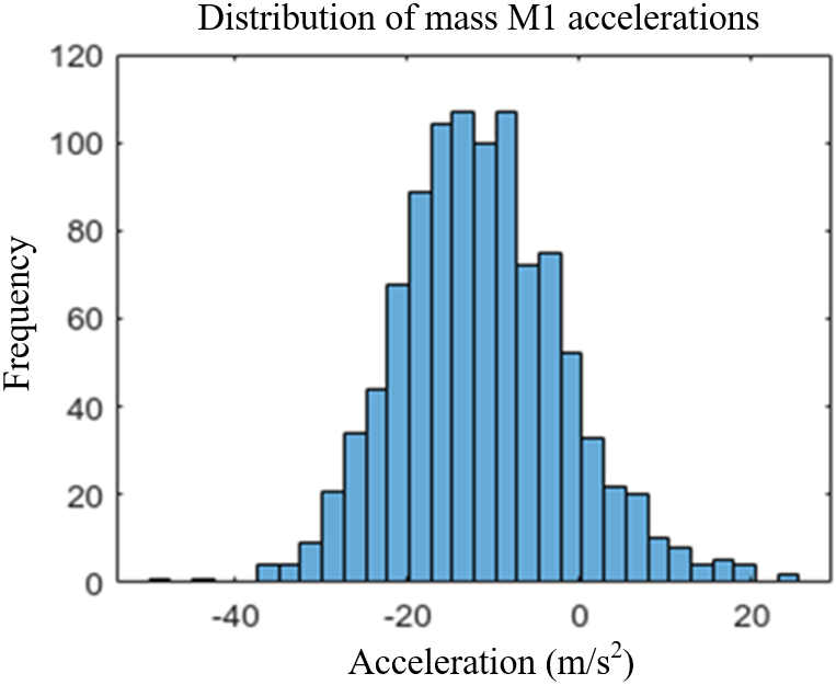 | 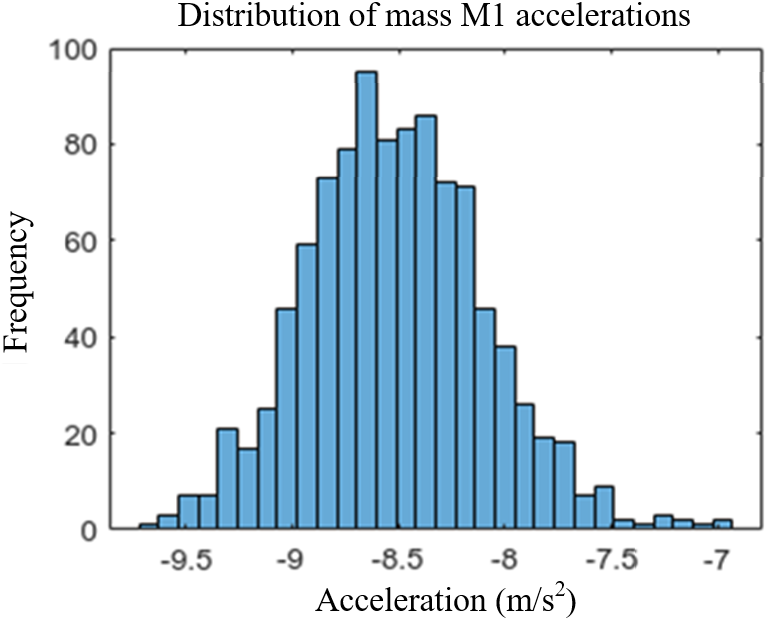 |
Distribution of M2 accelerations | 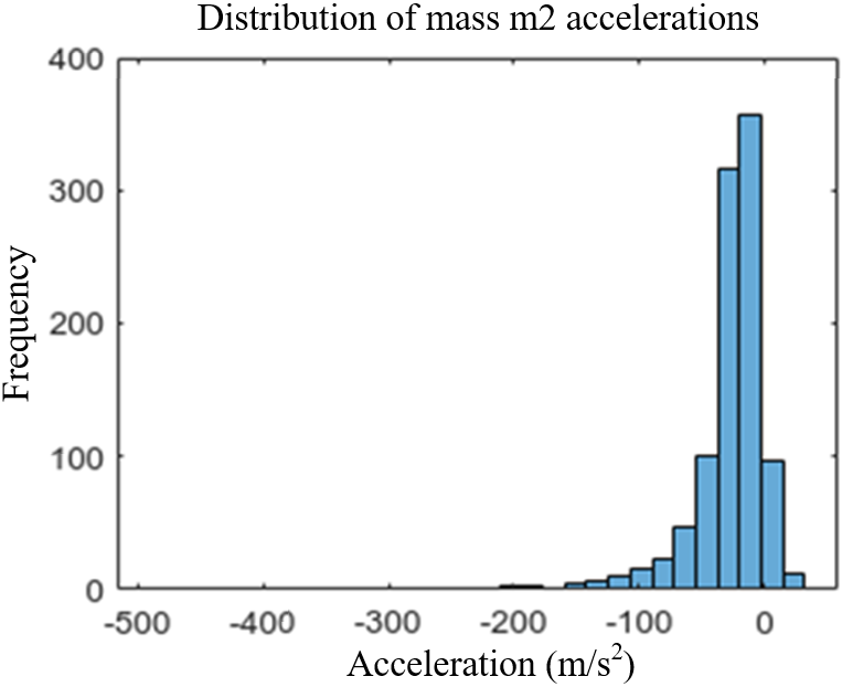 |  |
Average velocity variation for mass m2 over the time | 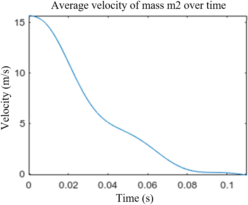 | 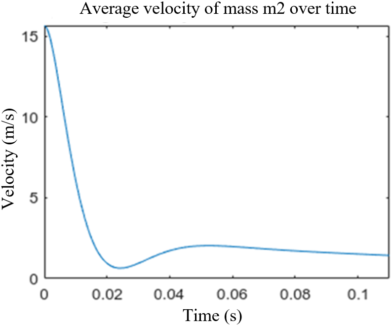 |
Weak Spring Constants | Strong Spring Constants | |
|---|---|---|
Simulation parameters | mean_c1 = 167000; std_c1 = 10000; mean_c2 = 8000; std_c2 = 1500; mean_k1 = 995790; std_k1 = 200000; mean_k2 = 779080; std_k2 = 15000 | mean_c1 = 167000; std_c1 = 10000; mean_c2 = 8000; std_c2 = 1500; mean_k1 = 3695790; std_k1 = 200000; mean_k2 = 2879080; std_k2 = 15000 |
Average deceleration | Average Mass M1 Acceleration: -18.003677 $\mathrm{m} / \mathrm{s}^2$ Average Mass m2 Acceleration: -17.010079 $\mathrm{m} / \mathrm{s}^2$ | Average Mass M1 Acceleration: -3.149762 $\mathrm{m} / \mathrm{s}^2$; Average Mass m2 Acceleration: -7.202527 $\mathrm{m} / \mathrm{s}^2$ |
Distribution of M1 accelerations | 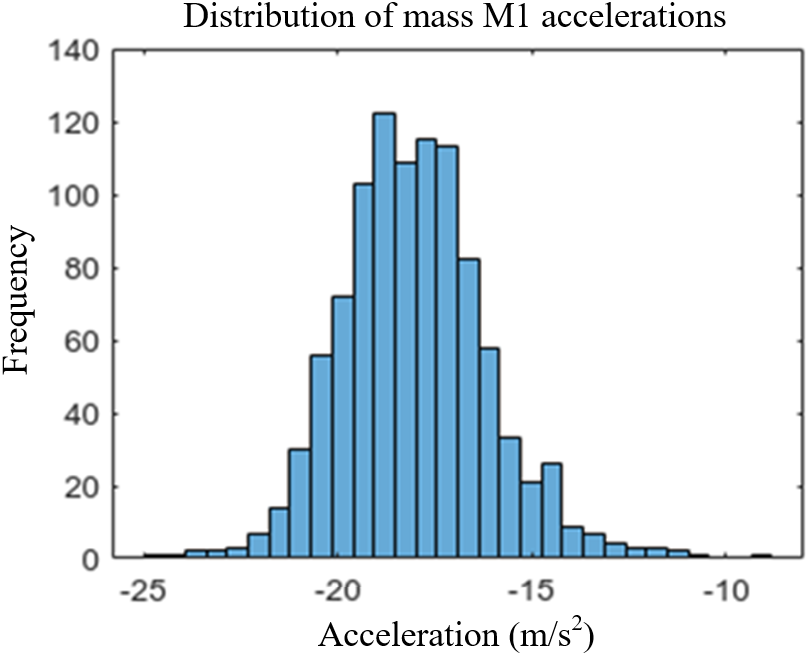 | 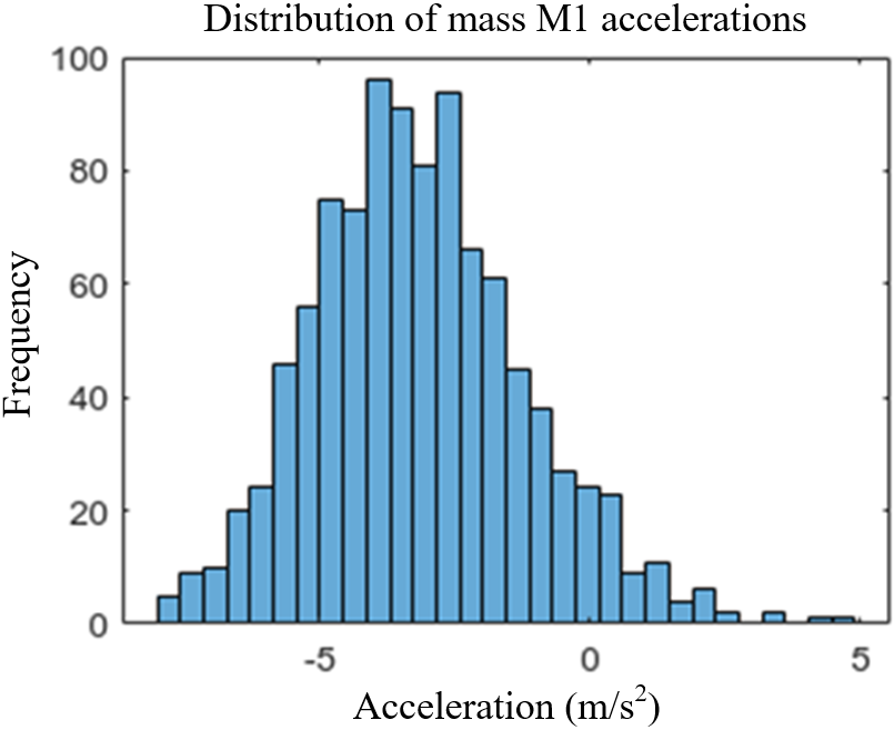 |
Distribution of M2 accelerations | 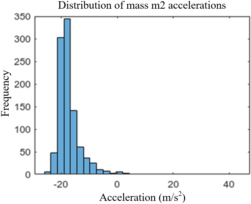 | 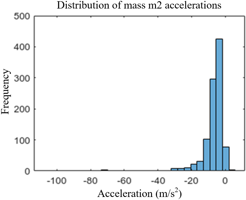 |
Average velocity variation for mass m2 over the time | 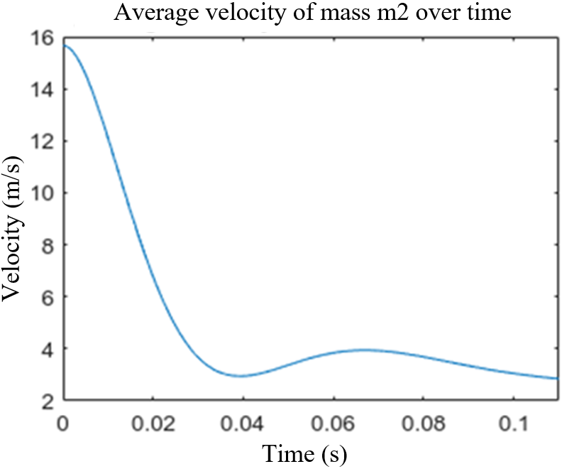 |  |
Based on Table 3, where the spring constants have been modified, the acceleration of two masses (M1 and M2) has been affected as follows:
With weak spring constants:
-Average Mass M1 Acceleration: -18.003677 $\mathrm{m} / \mathrm{s}^2$
-Average Mass M2 Acceleration: -17.010079 $\mathrm{m} / \mathrm{s}^2$
Lower spring constants (mean_k1 = 995790, mean_k2 = 779080) result in higher accelerations, indicating that the springs are less stiff and thus less effective at resisting deformation and absorbing shock.
With strong spring constants:
-Average Mass M1 Acceleration: -3.149762 $\mathrm{m} / \mathrm{s}^2$
-Average Mass M2 Acceleration: -7.202527 $\mathrm{m} / \mathrm{s}^2$
Higher spring constants (mean_k1 = 3695790, mean_k2 = 2879080) lead to significantly lower accelerations. This suggests that stiffer springs enhance the system’s ability to absorb impact without transmitting as much force to the masses, resulting in lower accelerations. Higher stiffness in springs reduces accelerations, which suggests that designing systems with higher stiffness could be advantageous for enhancing structural integrity and reducing the effects of sudden impacts.
4. Conclusion
This study developed a two-mass model with dual springs and dampers to simulate vehicle collisions, focusing on the impact of spring stiffness and damping on forces experienced during crashes. The model was validated with crash test data from a 2023 Honda Accord LX 4-Door Sedan, where vehicle acceleration was calculated from observed deformations and confirmed by deceleration sensors.
The equations of motion were derived and solved using state variables and the Laplace transform, with particular attention to energy transitions during collisions.
Parametric regression optimization integrated experimental and simulation data, resulting in a high-fidelity model. This alignment was demonstrated by the consistency between calculated and observed acceleration profiles, as well as velocity trends.
Key findings include that the chosen model, despite its simplicity, can accurately predict collision behavior when the appropriate parameters (k1, k2, c1, and c2) are selected. By utilizing vehicle crash test data and Monte Carlo simulations, we analyzed how these parameters influence dynamic responses. The optimization of these parameters can significantly reduce accelerations, thereby protecting both occupants and the vehicle structure. This underscores the importance of carefully selecting and tuning these parameters in vehicle frameworks. However, achieving a balance between stiffness for safety and ride comfort remains critical, necessitating a nuanced approach to vehicle design.
Overall, this research demonstrates that optimizing damping and stiffness in vehicle design can enhance crash safety. The insights gained validate the proposed model and provide actionable guidance for future vehicle design and safety standards, laying a solid foundation for ongoing innovation in automotive safety technologies aimed at significantly improving occupant safety in vehicular accidents.
The data utilized in this article can be accessed from the NHTSA database, specifically Test 15005.
The authors declare that they have no conflicts of interest.
