
Acadlore takes over the publication of JCGIRM from 2022 Vol. 9, No. 2. The preceding volumes were published under a CC BY license by the previous owner, and displayed here as agreed between Acadlore and the owner.
Determinates of Commercial Banks Liquidity: Internal Factor Analysis
Abstract:
This study was undertaken to explore the determinants of liquidity in Zimbabwean commercial banks. The research paper was motivated by the persistent high liquidity crunch currently be delving operations of commercial banks. An explanatory research design was adopted to find out variables that determine banks liquidity. An Ordinary Least Squares (OLS) model was developed after testing the variables for stationary to avoid spurious regression using the Augmented Dicker-Fuller (ADF) unit root test. Pearson’s correlation analysis was used to examine the existence of correlation between the repressors and the regressed. The study identified that non-performing loans are highly negatively related with banks liquidity signifying that this variable influence bank liquidity to a larger extent. A positive relationship between bank size and capital adequacy ratio and liquidity was established. Contrary to expectations a positive relationship was obtained between loan growth and banks liquidity. The following recommendations were made. Banks should devise robust credit risk management tools to reduce credit risk, tap into the offshore markets to obtain more credit to extent to their clients and the central banks should speed up the operation of ZAMCO which is meant to take over banks bad debts.
1. Introduction
According to the Bank for International Settlement (2009) many banks struggled to maintain adequate liquidity during the 2007-2009 Global Financial Crisis. The same phenomenon is being experienced in Zimbabwe since 2009 when the country adopted multiple currencies to address several macroeconomic challenges among them hyperinflation, volatile exchange rates and high interest rates.The multi-currency era has brought significant changes in market conditions and thus the importance of prudential liquidity risk measurement and management. A number of commercial banks are experiencing funding risk as they are unable to raise cash or cash equivalents to finance their operations either through the sale of money market instruments or borrowing from the Central Bank.
The situation is being aggravated by the absence of the Lender of Last Resort (LOLR), inactive money market, lack of confidence in the financial sector (resulting in mattress banking-an estimated \$3 billion is circulating outside the banking system), uncertain political environment and difficulties in sourcing external lines of credit due to perceived country risk. Moreso, some of the banks are still failing to meet the regulator’s minimum capital requirements. As at 30 June 2014, five out of nineteen banking institutions were undercapitalised; this translates to 26 percent (RBZ, MPS July 2014).
As financial intermediaries, banks play a pivotal role in driving the economy. Citing (Levine, 1996)Demirguc-Kunt and Huizinga (1998) opines that the efficacy of financial intermediation affect economic growth. This is achieved by channelling funds from surplus to deficit units in the economy. This view is supported by Sarr & Lybek (2002) who asserts that liquid markets are desirable for economic growth because; a) they facilitate central banks to indirectly transmit its monetary policy instruments to fine tune the economy to a desired state b) allow banks and other financial institutions to make money through duration mismatch and c) enable investors to participate in financial markets easily by entering and exiting the market easily.
However, when banks lack the necessary liquidity to fund the corporate world economic slowdown is usually experienced.According to Moore (2009) liquidity constrained banking systems might hinder economic activity as banks reduce lending. This may lead to company closures, reduced consumption, diminishing aggregate demand and higher unemployment (Bemanke, 1983). As concurred by Biyam (2010) business activity is slowed down as companies fail to restock, pay for their daily expenses and meet maturing obligations.
A reduction in funding by banks has seen the Zimbabwe’s economic growth contractingto 3.7 percent in 2013 from an estimated 4.4% in 2012 (AfDB, 2014). Moreso, capacity utilisation has fallen to around 36 percent from a peak of over 50 percent in 2009 (ZNCC, 2014). As a result of this economic stagnation a number of banks have been exposed to default risk. Similarly, in the US, in the aftermath of the Global Financial Crisis (GFC) commercial banks were exposed to Asset & Liability mismatch on both Balance Sheetand Off-Balance Sheet activities (Brunnermeier, 2009). The result was catastrophic. Several banks went under, with the contagion effect being felt world over as the“global recession”.
This shows that liquidity of commercial banks is fundamental to both the local economy and the world at large. This is aggravated by the roles played by banks in the economy apart from credit extension. They form the nerve centre of the economy hence the study of liquidity determination is of focus by academics, practioners and regulators.
Studies on the determination of bank liquidity are still very few save for studies such as; Valla et al (2006), Vodova(2011), Moore (2009), Raunch (2010), Fadare (2011), Tseganesh (2012) andChagwiza (2014). To my knowledge, no study has been undertaken to empirically explore bank specific factors that influence liquidity hording. This study adds foregoing discussions by filling this gap in Sub Saharan Africa. Another interest to this research is the unavailability of the Lender of Last Resort function in the Zimbabwean context.
Panel regression analysis methodology was employed to identify the key determinants of banks liquidity in Zimbabwe using a case study of NMB Bank for the period 2009-2014.
The rest of the paper is structured as follows. Section 2 focus on the review of related literature, Section 3 highlights the methodology adopted for this study, while, Section 4 presents the results. Section 5 makes conclusions and recommendations.
2. Literature Review
The concept of bank liquidity is elementary in financial markets. It represents a desirable function that should reflect a well organised financial market. Gabrielsen et al (2011) define a liquid market as “a state of condition when prevailing structure of transactions provide a prompt and secure link between the demand and supply of assets, thus delivering low transaction costs.” On the other hand, Borio (2009) defines market liquidity as the ability to trade an asset or financial instrument at short notice with little impact on its price.
From the above definitions it can be noted that liquid financial markets are characterised by low transactional costs, easy entry and exit and timely settlement. In most cases market liquidity is gauged by the liquidity of the individual assets in the market. However, Barker (1996) argues that there is no single unambiguous, theoretically correct or universally accepted definition of liquidity. According to the author this is so because some of the important characteristics of liquidity may change over time. From the views of Sarr & Lybek (2002) in good times, liquidity may primarily reflect transaction costs and in bad times, instantaneous price discovery and adjustment to a new equilibrium becomes essential.A bank’s liquidity is derived from its Balance Sheet. Moore (2009) discusses the Stock and Flow approach to liquidity measurement. The former utilises balance sheet ratios to identify liquidity movements within a bank. These ratios are:
i. Loan-to-Deposit (LD) ratio
ii. Short-term investments to Total Assets ratio
iii. Liquid asset ratio.
Vodova(2011) provide four Balance Sheet ratios used to measure a bank’s liquidity. The ratios discussed are:
Rule of Thumb: The higher the share of liquid assets to total assets, the higher the absorption capacity of liquidity shocks. However, high value of this ratio may be interpreted as inefficiency due to the lower returns on very liquid assets, hence the need of liquidity-profitability trade off.
Rule of Thumb: The acceptable ratio is 100% or more. This ratio signifies the ability of a bank to meet its funding needs.
Rule of Thumb: The higher the ratio the less liquid the bank is. This ratio measures the share of loans in total assets. It indicates the proportion of bank’s assets being tied up in loans.
Rule of Thumb: The higher the ratio the less liquid the bank is. This ratio relates to illiquid assets to liquid liabilities. The more illiquid assets it has to liquid liabilities the more prone it is to liquidity risk.
Berrospide (2013) investigated the causes of US banks to hoard liquidity during the recent global financial crisis using regression analysis. Liquidity hoarders were defined as those banks with an average ratio of total liquid asset to total assets which increased by more than 3% post crisis to the crisis period. The author employed a regression framework similar to Cornett et al (2011) to measure liquidity risk. The researcher found that stable funding sources such as bank deposits and capital are the main determinants of liquidity holding and liquidity holding decrease with bank size. Furthermore, in support of the precautionary motive to hold cash, the study revealed that US banks choose to build up liquidity buffer to cushion themselves against expected losses from securities write downs.
Bonner et al (2013) investigated the determinants of banks liquidity holdings using bank specific variables for 30 OECD countries. Their study revealed that without liquidity regulation, banks liquidity holding is determined by a combination of bank specific (business model, profitability, deposit holdings and size) and country specific (disclosure requirements, bank concentration) factors.
Jordan et al (2013) utilised the Vector Autoregressive methodology to analyse liquidity trends in the Bahamas over the period 2001 to 2011. The author noted that excess reserves are positively related to net domestic assets and negatively related to private sector credit and the Treasury bill rate (using the 1st model). The 2nd model showed that all the variables (net domestic assets, Treasury bill rate, ceiling on lending rate and real Gross Domestic Product) were all significant in explaining the excess reserve built up, except for private sector credit.
Tseganesh (2012) studied the determination of commercial banks liquidity in Ethiopia for the period 2000 to 2011.The author went on to analyse the effects of banks liquidity on profitability. Balanced fixed effect regression was used on eight commercial banks. The results show that capital adequacy, bank size, share of non-performing loans to total loans, interest margins, inflation rate and short term interest rates are statistically significant to explain banks liquidity, contrary to Vodova(2011). More so, Real GDP growth rate and loan growth were found to have a significant impact on bank liquidity.
Wuryandani (2012) investigated the determinants of banks liquidity using longitudinal panel data of individual Indian banks for the period January 2002 to November 2011. The researcher utilised the Generalised Method of Moments (GMM) simultaneous equation methodology. Results indicate that credit, savings and deposit affect precautionary liquidity, whilst financial system and macroeconomic conditions affect involuntary liquidity.
Fadare (2011) sought to assess the development and impact of Nigerian banking liquidity regulations, identify the key determinants of banking sector liquidity in Nigeria and explore the effects financial crisis on the banking sector liquidity regulations. Leveraging on theoretic considerations, the author came up with an Autoregressive Ordinary Least Squares specification. The study showed that in the absence of financial crisis, banks either hold excess liquidity or hold liquidity in line with regulatory requirements. On the contrary,during episodes of financial crisis banks were found to behighly illiquidrelative to benchmarks thereby exposing themselves to financial distress. These results are similar to Vodova (2011)
Moore (2009) explored the main determinants of bank liquidity and also evaluated the impact of banking crisis on liquidity. Using evidence from Latin America and the Caribbean the author found that on average, bank liquidity is about 8% less than what is in line with economic fundamentals during crisis.
The same author provided an assessment of whether behavioural models, linear time series or non-linear time series models are better able to account for liquidity dynamics during a crisis. Employing monthly observations for sixteen Latin America and Caribbean nations for the period 1970 to 2004, the author found that behavioural models performed exceptionally well in predicting liquidity trends during the crisis in Argentina, Bolivia, Paraguay and Venezuela in both the short and long run.
Vodova (2011a) studied the determinants of liquidity of Slovak commercial banks using bank specific and macroeconomic data from 2001 to 2010. The author employed panel data regression analysis. Results revealed that bank liquidity drops mainly as a result of financial crisis, bank liquid assets also drop with higher profitability, higher capital adequacy ratios and the size of the bank. On the other hand liquidity measured by lending activity of banks is positively related to GDP growth and bank profitability, but negatively related to high levels of unemployment. The following variables; level of interest rates, interest spreads, inflation rate and the level of non-performing loans were found to be of no significance in the determination of Slovak commercial banks.
The same author in (2011b) analysed the determinants of commercial banks liquidity of Czech commercial banks for the period 2001 to 2009. Using panel regression analysis, the author identified a positive link between bank liquidity and capital adequacy, share of non-performing loans and interest rates on loans and interbank transactions contrary to his earlier findings for the Slovak banks. These variables; inflation rate, business cycles and financial crisis had negative effect on liquidity. Based on the findings, the author concluded that the relation between bank size and liquidity is ambiguous.
Aspachs et al (2005) provides a comprehensive analysis of the determinants of UK banks liquidity policy over the period 1985 to 2003. Their study was aimed at investigating how central bank lender of last resort policy affects banks liquidity holding. They found that the greater the likely support from the central bank in the event of a liquidity crisis, the lower the liquidity buffer that banks hold.
3. Research Methodology & Data
This study focused on bank specific variables that determine banks liquidity with a case study of NMB Bank Zimbabwe. This bank was chosen because of data availability(all its financial statements post dollarisation (2009) are publicly available). Following Tseganesh (2012) in order to identify the determinants of liquidity of Zimbabwean commercial banks, initially descriptive statistics were analysed. An Ordinary Least Squares (OLS) model was developed after testing the data for stationarity to avoid spurious regression using the Augmented Dicker-Fuller (ADF) unit root test. The model was tested for adequacy by carrying out tests of OLS assumptions. Pearson’s correlation analysis between the regressors and the regressand was made. Semi-annual data was used in this study which was obtained from the NMB banks’ financial statements for the period 2009 to 2014. The data was analysed using Eviews 7 econometric software package.
Banks liquidity was measured using liquidity ratio L3 described above. The following longitudinal regression model was estimated;
Where: Lit = liquidity ratio L1 and L3 for bankt in timet
Xit = vector of explanatory variables for bankt in timet
𝛽 = coefficient which represents the slope of variable
𝛼 = constant
𝜀𝑖t = error term
Incorporating bank specific variables into the modelyield:
Where: Lit = liquidity ratio L1 and L3 for bankt in timet
𝛽1…4=Coefficient which represents the slope of variable
CARit = is the capital adequacy ratio for bank i in period t, proxied by the ratio of equity to total assets i.e.
$C A R_{i t}=\frac{\text { EQUITY }}{\text { TOTALASSETS }}$ (+)
SIZEit = is the size of bank i in period t, proxied by the natural logarithm of a bank’s total assets i.e.
SIZE=LN(TOTALASSETS) (+)
LGit = is the growth in loans for bank i in period t, proxied by the natural logarithm of percentage in loans & advances to customers i.e.
$L G=\ln \left(\frac{\text { LOANS\&ADVANCES }_t}{\text { LOANS\&ADVANCES }_{t-1}}\right)$ (-)
NPLit = is the non-performing loan of bank i in period t, proxied by the share of non-performing loan from the total loan portfolio of a bank i.e.
$N P L=\left(\frac{\text { NONPERFOMINGLOANS }}{\text { TOTALLOANS }}\right)$ (-)
4. Results& Their Discussion
CAR | LG | LIQRATIO | NPL | SIZE | |
Mean | 18.35455 | 0.636364 | 0.792727 | 15979868 | 18.63909 |
Median | 17.28000 | 0.270000 | 0.820000 | 8983037. | 18.94000 |
Maximum | 38.00000 | 3.950000 | 1.000000 | 41877499 | 19.39000 |
Minimum | 10.66000 | 0.010000 | 0.530000 | 8420.000 | 17.03000 |
Std. Dev. | 7.655145 | 1.130701 | 0.163346 | 16965553 | 0.808980 |
Skewness | 1.697885 | 2.573325 | -0.500929 | 0.540984 | -0.864128 |
Kurtosis | 5.061145 | 8.147894 | 1.972540 | 1.640358 | 2.477819 |
Jarque-Bera | 7.232305 | 24.28654 | 0.943889 | 1.383836 | 1.493956 |
Probability | 0.026886 | 0.000005 | 0.623788 | 0.500615 | 0.473796 |
Sum | 201.9000 | 7.000000 | 8.720000 | 1.76E+08 | 205.0300 |
Sum Sq. Dev. | 586.0125 | 12.78485 | 0.266818 | 2.88E+15 | 6.544491 |
Observations | 11 | 11 | 11 | 11 | 11 |
The banks mean (average) capital adequacy ratio (CAR) since dollarisation was estimated to be 18.35 percent against the regulator’s 12 percent threshold. Using this ratio to reflect the bank’s capitalisation, NMB is fairly capitalised. Loan growth is faring well with an average growth of 63.63 percent. However, despite this good performance, the non performing loans (NPL) figure is not pleasing. Although the bank has been very aggressive in dishing out loans it remains challenged in recovering loaned out monies. The NPL figure grew from a tiny $8,420 in 2009 to a staggering $41,977,499 by the first half of 2013. The bank attributed this phenomenal jump in NPLs to economic stagnation and liquidity problems currently bedelving the nation. On theother hand, the bank’s liquidity ratio which averaged 79.27 percent is very high. This ratio indicates the proportion of the bank’s assets being tied up in loans. In this case 79.27 percent of the bank’s total assets are tied in illiquid assets (loans).
VARIABLE | ADF STATISTIC | CRITICAL VALUE | ORDER OF INTEGRATION |
DECISION | SIGNIFICANCE LEVEL |
LIQ Ratio |
-6.534114 | -4.582648 -3.320969 -2.801384 |
Level |
Stationary | 1% 5% 10% |
CAR |
-4.581405 | -4.297073 -3.212696 -2.747676 | Level |
Stationary | 1% 5% 10% |
LG | -17.28981 | -5.295384 -4.008157 -3.460791 | Level |
Stationary | 1% 5% 10% |
NPL |
-11.76721 | -3.007406 -2.021193 -1.597291 | Level |
Stationary | 1% 5% 10% |
SIZE |
-6.372984 | -4.297073 -3.212696 -2.747676 | Level |
Stationary | 1% 5% 10% |
All the variables are stationary in levels at 1 percent significance level. This means all the variables have no unit roots hence they are stationary which is a prerequisite condition to run a good regression model.
Variable | Coefficient | Std. Error | t-Statistic | Prob. |
|
|
|
|
|
|
|
|
|
|
C | -9.461712 | 2.693476 | -3.512826 | 0.0126 |
CAR | 0.020429 | 0.010499 | 1.945730 | 0.0996 |
LG | 0.012798 | 0.054574 | 0.234516 | 0.8224 |
NPL | -1.58E-08 | 5.07E-09 | -3.119812 | 0.0206 |
SIZE | 0.543163 | 0.140793 | 3.857873 | 0.0084 |
|
|
|
|
|
|
|
|
|
|
R-squared | 0.779521 | Mean dependent var | 0.792727 | |
Adjusted R-squared | 0.632536 | S.D. dependent var | 0.163346 | |
S.E. of regression | 0.099018 | Akaike info criterion | -1.484069 | |
Sum squared resid | 0.058828 | Schwarz criterion | -1.303208 | |
Log likelihood | 13.16238 | Hannan-Quinn criter. | -1.598077 | |
F-statistic | 5.303379 | Durbin-Watson stat | 2.274248 | |
Prob(F-statistic) | 0.035782 | |||
The table above shows the results of the regression model. The liquidity ratio (proxy for bank liquidity) is the dependent variable which is taken to be influenced by nonperforming loans (NPL), capital adequacy ratio (CAR), loan growth (LG) and bank size (SIZE). Looking at the significance of the regressors the author note that NPL and SIZE have p-values of 2.06 percent and 0.84 percent respectively. They are significant in explaining banks liquidity. Since 50 percent of the regressors are significant this model is good. The R2 is 78 percent and the adjusted R2 is 63 percent which is above 60 percent; therefore, we can note that the data is fitted properly. The F statistic is significant with a p-value of 3.58 percent. This means the regressors jointly can influence the independent variable.
Given that the model is good, the following regression equation was estimated:
$L_{N M B t}=-9.461712+0.0204 C A R_{N M B t}+0.5432 S I Z E_{N M B t}+0.0128 L G_{N M B t}$
$-1.58 E-08 N P L_{N M B t}+\varepsilon_{N M B t}$
The intercept (𝛽0) has a coefficient of -9,461712. This means taking the regressors to be zero we expect bank liquidity to be -9,461712 units. This holds for Zimbabwe since the country is faced with a liquidity crunch we expect the intercept to be negative. Capital adequacy ratio has a correlation coefficient of 0,0204 indicating that a 1 percent increase/decrease in capital adequacy ratio translates to 2,04 percent increase/decrease in bank liquidity. Although this coefficient is positive it has a weak explanatory power suggesting that it is not a good indicator of liquidity position of a bank. These results are consistent with Tseganesh (2012) and Vodova (2011) but contrary to the findings of Berrospide (2013) who argue that liquidity holding decrease with bank size.
Commenting on loan growth a correlation coefficient of 0,0128 was established, meaning a 1 percent increase/decrease in loan growth translate to 1,28 percent increase/decrease in bank liquidity. Contrary to expectations this relationship was found to be positive along the lines of Tseganesh (2012). This can be explained by the huge appetite for loans currently obtaining in Zimbabwe whereby loan growth is growing spontaneously with bank liquidity.
A negative correlation coefficient of -1,58E-08 between non performing loans and liquidity position of banks was determined. This suggests that a 1 percent decrease/increase in nonperforming loans causes bank liquidity to increase/decrease by 158 percent. This holds in reality because if a bank fails to collect outstanding loans this scare away depositors hence its liquidity suffers. As expected the nonperforming figure is a significant determinant of bank liquidity in Zimbabwe in the multiple currency era. Tseganesh (2012) and Vodova (2011) oppose these results.
Bank size was found to have a correlation coeffient of 0.5432 indicating that a 1 percent increase/decrease in bank size cause the liquidity position of a bank to increase/decrease by 54,32 percent. This is consistent with our expectations as suggested in section III of the study. These results are in harmony with Bonner et al (2013) and Tseganesh (2012). In relation to the traditional transformation view a positive relationship should exist between bank size and liquidity as indicated in these results.
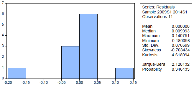
The normality test was carried out using the Jarque-Bera test. The p-value was established to be 34.64 percent which is greater than 5 percent (significance level). Since the p-value is greater than 5 percent, the null hypothesis that residuals are normally distributed cannot be rejected. Therefore the residuals are normally distributed.
Breusch-Godfrey Serial Correlation LM Test:
| F-statistic | 0.125305 | Prob. F(2,4) | 0.8856 |
| Obs*R-squared | 0.648544 | Prob. Chi-Square(2) | 0.7231 |
Using the Breusch-Godfrey Serial Correlation test to test for serial autocorrelation in the residuals, a p-value of 72.31 percent was determined. The null hypothesis that residuals are not serially correlated cannot be rejected. For this model the residuals are not serially correlated.
| Heteroskedasticity Test: Breusch-Pagan-Godfrey | |||
| F-statistic | 0.217235 | Prob. F(4,6) | 0.9194 |
| Obs*R-squared | 1.391531 | Prob. Chi-Square(4) | 0.8457 |
| Scaled explained SS | 0.748962 | Prob. Chi-Square(4) | 0.9452 |
This test was conducted using the Breusch-Pagan-Godfrey test. A p-value of 84.57 percent was estimated; therefore the null hypothesis that residuals are homoskedasticity cannot be rejected. In light of these results the residuals are homoskedasticity which is good for our model.
5. Conclusion
The aim of this paper was to explore the determinants of commercial banks liquidity in Zimbabwe in the multiple currency era. A case study of NMB bank was used as the sample for the study. Panel data was analysed for the period 2009:Q1 to 2014:Q1.
The study revealed that non performing loans are strongly negatively related with banks liquidity. It follows that as non performing loans rise banks liquidity deteriorates. A positive relationship was identified between bank size and liquidity. In line with theory big banks are expected to be more liquid than smaller ones. A weak positive relationship was obtained between capital adequacy ratio and banks liquidity signifying that in Zimbabwe capital does not play a role in explaining banks liquidity. On the other hand, contrary to expectations loan growth was found to be positively related to banks liquidity although the relationship is very weak. This can be explained by the huge appetite for loans in Zimbabwe by economic agents.
The paper makes the following recommendations. Commercial banks should come up with robust credit risk management tools to reduce non performing loans. More so, domestic banks should look for ways to tap into the diaspora market to obtain more credit lines which will boost their liquidity positions. The central bank should speed up the operation of Zimbabwe Asset Management Company (ZAMCO) that has been established to take up bad debts in banks loan books. The study advocates other authors to look at a comprehensive study which incorporates more banks into the study using descriptive survey methodology since this study used a case study of one bank.
The data used to support the findings of this study are available from the corresponding author upon request.
The authors declare that they have no conflicts of interest.