Acadlore takes over the publication of JCGIRM from 2022 Vol. 9, No. 2. The preceding volumes were published under a CC BY license by the previous owner, and displayed here as agreed between Acadlore and the owner.
Volatility Spillovers and Stock Market Co-Movements Among Western, Central and Southeast European Stock Markets**
Abstract:
The aim of this paper is to examine the return and volatility spillovers and stock market co-movements among Western, Central and Southeast European stock markets. To examine the volatility spillover effects we employ a multivariate GARCH-BEKK (1, 1) model on a daily data from 2005 to 2014. There is a high and stable conditional correlation between Central and Western European markets during most of the analyzed period and the conditional correlation rises sharply during the periods of financial turmoil, suggesting some evidence on contagion. Conditional correlation between Croatian and Romanian markets and their Western counterparts is modest but it increases during the periods of financial crisis. Conditional correlation coefficients indicate that Macedonian and Serbian stock markets are relatively isolated from the advanced European markets. The return spillovers are investigated with the forecast-error variance decomposition based on the generalized VAR model. Following Diebold and Yilmaz (2012), we develop “spillover indices” based on the variance decomposition results on the generalized VAR model. The results indicate that total spillover index rose sharply during the periods of major financial disruptions. DAX and FTSE100 are the major net transmitters of spillovers to Central and Southeast European markets. There are bi-directional spillovers between DAX and FTSE100, between PX and WIG-20 and between MBI10 and BELEX15.
1. Introduction
The “financial contagion” phenomenon is one of the most exploited topics in the modern finance. After the US stock market crash from the 1987 and the emerging-market crisis during the 1990s, the economists developed many theoretical concepts to explain this phenomenon. The economists were particularly interested to explain how country-specific shocks were transmitted to the countries that are geographically distant, have different economic and financial structures and countries that don’t exhibit significant economic and financial links (Forbes and Rigobon, 2008; Pericolli and Sbracia, 2001). In other words, financial contagion means that increased volatility cannot be explained by macroeconomic fundamentals (Pericoli and Sbracia, 2001). By macroeconomic fundamentals in the sense of the contagion phenomenon, the economists commonly refer to the trade, financial and economic linkages which are normally responsible for transmissions of shocks among financial markets (Dungey, 2003; Jing 2013). There are two common characteristics of the contagion phenomenon- volatility spillovers and increased co-movements among financial markets during the periods of financial disruption. The degree of stock market co-movements have very important implications for the international investors. If the stock market co-movements are small, international investors could diversify their portfolios while reducing the overall portfolio risk. While the stock market co-movements tend to increase during the periods of financial turbulence, the benefits of diversification become smaller. Many authors tried to explain the financial contagion with psychological elements. Among one of the most popular theories trying to explain this phenomenon is the theory that suggests that contagion occurs as a result of the herding behaviur (Cipriani and Guarino 2001, Cheung et.al 2009). Herding behavior theory assumes that market participants have asymmetric information. When there are turbulences in one of the markets, market participants tend to revaluate other markets based in their limited information.
Some authors explain the financial contagion using the “wake-up call” hypothesis. When one of the countries experiences financial crisis or financial disruptions, investors from the other countries tend to reexamine the stability of their home countries and they might develop expectations of a future financial crisis in their home countries. King and Wadhwani (1990) explained the volatility spillovers after the US stock market crash with their “information correlation” theory. Kodres and Pritsked (2002) examined the portfolio channel of financial contagion. When the investors from one country are hit by idiosyncratic shock, they tend to rebalance their portfolios through other countries in order to adjust their risk.
There are several different approaches to measure the “contagion” effect. One of the most popular techniques was the “correlation approach” developed by Forbes and Rigobon (1999). This approach measures the correlation between the stock market returns during the “tranquil” periods and crisis periods. Most of the research is based on multivariate GARCH models and their extensions. Some of the researchers also use VAR models and cointegration technique to analyze the spillover effects.
There is a vast literature analyzing the contagion in the case of developing and emerging markets. However, there are only a few papers that examine the volatility spillovers and stock market co-movements in the case of Central and Southeast European countries. The aim of this paper is to examine the time-varying stock market correlations and return and volatility spillovers among Western European and Central and Southeast European countries. Conditional correlation plots will be estimated based on the results from multivariate GARCH BEKK (1, 1) model. We are particularly interested to examine whether the conditional correlation increases significantly during the period of the global financial crisis and European debt crisis. Volatility spillovers will be examined from the coefficients of the estimated GARCH BEKK model. To examine the return spillovers, we will create spillover index based on generalized VAR framework developed by Diebold and Yilmaz (2012).
2. Literature Review
The correlation approach was introduced by Forbes and Rigobon in 1999. Their approach shows that previous findings of increased co-movements during the crisis periods were biased. Their results show that increased co-movements during the crisis periods are conditional of increased volatility and some authors misinterpreted these findings as an evidence of contagion. Their approach can calculate cross-market correlations while correcting for the heteroskedasticity. Forbes and Rigobon (1999) conclude that there is no evidence of contagion during the Asian crisis, Mexican crisis and 1987 US stock market crash.
While the Forbes-Rigobon (1999) method corrects for the heteroskedasticity, it doesn’t control for the volatility clustering phenomenon. Dungey (2005; 2010) introduced a model that accounts for the volatility clustering. Opposite of the Forbes and Rigobon (1999), Dungey (2010) finds evidence of contagion across the analyzed markets.
Gravelle et.al (2006) extented the Forbes-Rigobon approach to allow for regime switching volatility. Their approach can detect regime changes using the Markov regime-switching model. Unlike the Forbes-Rogobon approach where we need to know the source (country) of the specific shock, this approach allows financial disruptions to be driven by large common shocks.
Favero and Giavazzi (2002) use VAR model to test for contagion during the ERM currency crisis. They find evidence of contagion among the six ERM countries (France, Italy, Spain, Belgium, Holland and Denmark). Diebold and Yilmaz (2009; 2012) developed the return and volatility “spillover index” based on the forecast error variance decompositions on a generalized VAR model. In the recent period, this approach is widely used to analyze return and volatility spillovers among stock markets, bond markets and currency markets (Claeys and Vasicek, 2014; Louzis, 2013; Suwanpong 2011). Alter and Bayer (2013) use a VAR with exogenous variables (VARX) model and a generalized VAR framework proposed by Diebold and Yilmaz (2012) to create so called “contagion index”. Their results show evidence of significant spillovers from the sovereign credit crisis to the euro-zone banking system.
However, most of the researchers used multivariate GARCH models to examine volatility spillovers across the stock markets. Echner (2006) used the DCC-GARCH model on the case of the stocks in the Dow Jones Industrial Avarage, and found statistically significant volatility spillovers among stocks.
Horvath and Petrovski (2012) examined the stock market co-movements between Western European stock markets and their Central and Southeast counterparts. They employed GARCH-BEEK model on the daily stock market data from 2006 to 2011. Their results suggest that Central European stock markets are strongly integrated with Western European markets. They found that conditional correlation between Central and Western European stock market varies around 0,6. Interesting, their results indicate that global financial crisis didn’t changed the value of conditional correlation. On the other side, Horvath and Petrovski (2012) found that correlation between Serbian and Macedonian vis-a-vis their Western counterparts fluctuates around zero. Croatia exhibits somehow higher correlation (particularly in the pre-crisis periods), suggesting that Croatia is financially more integrated than the Serbia and Macedonia. Horvath and Gjika (2012) also find strong stock market correlations between Central European and Euro-Area stock markets using assymetric DCC-GARCH model. Li and Majerowska (2006) used the GARCH-BEEK model and found evidence for volatility spillovers from developed markets to Hungary and Poland. The results from the variance decomposition suggest that only 20% of the variation of the returns in the Hungary and Poland can be explained by shocks from the developed markets.
Babecky et.al. (2008) examined the speed of convergence (β-convergence) and degree of financial integration (σ-convergence) between four Central European Countries and Euro Area. Their results suggest that Central European countries (except Slovakia) exhibit strong and significant correlation between stock market returns.
Analysis on more frequent intraday data can be found in Egert and Kocenda (2011). They use DCC-GARCH model and 5-minute intraday stock market prices for the period 2003-2006. Their results indicate strong correlation between developed Western stock markets (German, French and UK). On the other side, the correlation between Central (Poland, Hungary and Czech) and Western (Germany, France and UK) markets is small but it exhibits an upward trend.
3. Data
We use daily index values for the eight stock market indices: MBI10 (Macedonian stock exchange), WIG20 (Warsaw stock exchange), FTSE100 (London stock exchange), BET (Bucharest stock exchange), CROBEX (Zagreb stock exchange), BELEX15 (Belgrade stock exchange), DAX (Frankfurt stock exchange) and PX (Prague stock exchange). Data is collected for the period 04/10/2005- 03/03/2014 from the Quandl database and national stock market websites. Daily time-series on stock market prices are available in Figure 1. Series of daily returns are created as a logarithmic differences series on a daily index values (Figure 2). There are 1818 observations for each of the stock market indices. Descriptive stats for the daily return series are presented in table 1. All of the return series exhibit similar standard deviations in a range from 1,5% to 1,9%. JB values indicate that the stock markets returns series are not normally distributed (series exhibit fat tails and high peaks), which is a common characteristic of financial time series. As we can see from the Figure1, series on stock market returns exhibit volatility clustering, which is common for stock markets data- large stock market returns tend to be followed by large stock market returns and small returns tend to be followed by small stock market returns (Brooks, 2002). GARCH models can capture all of the characteristics that were mentioned above.
DAX FTSE100 PX WIG20 MBI10 CROBEX BET BELEX15 | ||||||||
Mean | 0.000335 | 9.99E-05 | -0.000217 | -2.94E-05 | -0.000219 | -0.000106 | 6.58E-06 | -0.000313 |
Median | 0.001262 | 0.000472 | 0.000323 | 0.000296 | -0.000479 | -4.98E-06 | 0.000495 | -0.000273 |
Maximum | 0.107975 | 0.096416 | 0.123641 | 0.108961 | 0.166301 | 0.147790 | 0.106994 | 0.140103 |
Minimum | -0.086140 | -0.092656 | -0.161855 | -0.116855 | -0.102831 | -0.107636 | -0.154782 | -0.125890 |
Std. Dev. | 0.015927 | 0.014321 | 0.017806 | 0.017943 | 0.015925 | 0.014995 | 0.019652 | 0.016836 |
Skewness | -0.028187 | 0.033319 | -0.472076 | -0.288982 | 0.677558 | -0.121056 | -0.867652 | 0.061047 |
Kurtosis | 10 | 11 | 15 | 7 | 18 | 17 | 13 | 19 |
Jarque-Bera | 3.236 | 4.940 | 1165,63 | 1.282 | 16479.90 | 14555,07 | 7.838 | 18371,73 |
Probability | 0.000000 | 0.000000 | 0.000000 | 0.000000 | 0.000000 | 0.000000 | 0.000000 | 0.000000 |
Observations | 1818 | 1818 | 1818 | 1818 | 1818 | 1818 | 1818 | 1818 |
4. Methodology
The families of ARCH and GARCH models are one of the most popular tools for modeling volatility. These models are designed to capture the specific characteristics of financial data: heteroskedasticity, volatility clustering, leptokurtosis and the leverage effects. The ARCH model was introduced by Engle (1982). The GARCH model was developed as a natural generalization of an ARCH model by Bollerslev (1986). Under the GARCH model, conditional variance depends on the long term average variance (v), volatility during the previous period (α) and the lagged term for the variance (β). GARCH (1, 1) model can be expressed as:
$\sigma_t^2=v+\alpha \varepsilon_{t-1+}^2 \beta \sigma_{t-1}^2$
There are many extensions of the standard GARCH models, designed to capture some of the specific characteristics of the analyzed financial data. The GJR-GARCH and EGARCH models were developed to account for the leverage effects (Brooks, 2002). GARCH-M (GARCH in mean) model adds a heteroskedasticity term in the mean equation (Su and Huang, 2010). The IGARCH (integrated GARCH) model is a strictly stationary variant of the GARCH model – it is a restricted version of the standard GARCH model. For more information about the different variants of GARCH models see Bollerslev et.al. (1992).
Multivariate GARCH models are designed to capture the co-movements (interdependence) of the financial asset returns and to capture the dynamics of the conditional variances and conditional covariances. As financial markets become more integrated, volatilities tend to move together over time. Also, there is often a “volatility spillover” across the financial markets – financial disruptions in a specific market are transmitted to other financial markets.
The mean equation in the multivariate GARCH models can be defined as:
$\boldsymbol{R} \boldsymbol{t}=\mu+u_t$
Bollerslev, Woolbridge and Engle (1988) developed the VECH model. The VECH model can be specified as:
$\operatorname{VECH}\left(H_t\right)=C+A \operatorname{VECH}\left(\varepsilon_t-1 \varepsilon_{t-1}^{\prime}-1\right)+B \operatorname{VECH}\left(H_{t-1}\right) \quad$ where
$C$ is an $N(N+1) / 2 \times 1$ parameter vector
A and $\boldsymbol{B}$ are $N(N+1) / 2 \times N(N+1) / 2$ matrices and
VECH – “operator that stacks the upper triangular portion of a symmetrical matrix” (Horvath and Petrovski, 2012 p.9)
So, the conditional variances and conditional covariances depend on the returns on the assets, the lags of the squared errors and on the lags of the conditional variances and conditional covariances between the asset returns (Brooks, 2002).
In order to ensure that H matrix is always positive definite, Baba, Engle, Kraft and Kroner (1995) introduced the BEKK model. The BEKK model can be specified as:
$H_t=C C^{\prime}+A^{\prime} H_t-1 A+B^{\prime} \varepsilon_t-1 \varepsilon_t^{\prime}-1 B$
where C is an upper triangular matrix of parameters. Matrix A measures the effects on the conditional variance from the own past shocks (innovations) and the effects from the past cross innovation from variable i to variable j. Diagonal elements of the B matrix measure the own volatility spillover effects, or effect from the past conditional variance (GARCH effects). The off-diagonal elements measure the cross-volatility spillovers among variables.
Multivariate GARCH models are commonly estimated with the Maximum likelihood function:
$\log L_t(\theta)=-\frac{N-T}{2} \log (2 \pi)-\frac{1}{2} \sum_{t=1}^T \log \left|H_t\right|-\frac{1}{2} \sum_{t=1}^T \varepsilon_t^{\prime} H t-1 \varepsilon_t$
In this paper, we will use the GARCH-BEKK model to estimate the volatility spillovers and stock market co-movements among eight different stock markets.
In order to examine the return spillovers among the eight stock markets we will create “spillover index” based on Diebold and Yilmaz (2009; 2012). Diebold and Yilmaz developed an intuitive measure for stock market interdependence to analyze the return and volatility spillovers across the stock markets. Since the estimated “spillover index” is time varying, we can see if there is any evidence of contagion during the recent financial crisis. This approach is based on the estimated VAR model, and the variance decomposition approach from the estimated VAR model. Firstly, we test the stationarity of the stock market indices using the Augmented Dickey-Fuller test. In their first paper, Diebold and Yilmaz (2009) use Cholesky decomposition and the results are very sensitive to the ordering of the variables. To overcome this limitation, Diebold and Yilmaz (2012) use variance decomposition based on generalized VAR, which is independent on the ordering of the variables. Here, we will also use the generalized variance decomposition.
Using the generalized VAR we will estimate the total spillovers index, directional spillovers and net spillovers among stock market indices.
Vector Autoregressive (VAR) models are developed by Sims (1980). Under the framework created by Sims the standard (covariance stationary) VAR model can be presented as:
$\boldsymbol{x}_t=\sum_{i=1}^p \boldsymbol{\Phi}_{\boldsymbol{i}} \boldsymbol{x}_{\boldsymbol{t - i}}+\boldsymbol{\varepsilon}_{\boldsymbol{t}}+$ and Et is a white noise process $\boldsymbol{\varepsilon} \sim(\mathbf{0}, \boldsymbol{\Sigma}).$
To get the variance decomposition estimations, we present the VAR model in a moving average form:
$x_t=A_1 \phi_{t-1}+A 2 \phi_{t-2}+\cdots . A p \phi_{t-p}$ and $A=0$ for $i<0$
To meet the stability conditions equation 1:
$\left|\boldsymbol{I}_n \lambda^p-\boldsymbol{\Phi}_{\mathbf{1}} \lambda^{p-1}-\boldsymbol{\Phi}_2 \lambda^{p-2}-\cdots-\boldsymbol{\Phi}_{\boldsymbol{p}}\right|=0$
As we noted earlier, Cholesky decomposition of the variance-covariance matrix makes the variance decomposition to be dependent on the ordering of the variables. Following Koop et.al (1996) H-step forecast error variance decomposition based on generalized impulse response functions can be estimated as:
$\theta_{i j}^g(H)=\frac{\sigma_{i i}^{-1} \sum_{h=0}^{H-1}\left(\boldsymbol{e}_{\boldsymbol{i}}^{\prime} \boldsymbol{A}_{\boldsymbol{h}} \boldsymbol{\Sigma} \boldsymbol{e}_{\boldsymbol{j}}\right)^2}{\sum_{h=0}^{H-1}\left(\boldsymbol{e}_{\boldsymbol{i}}^{\prime} \boldsymbol{A}_{\boldsymbol{h}} \boldsymbol{\Sigma} \boldsymbol{A}_{\boldsymbol{h}}^{\prime} \boldsymbol{e}_{\boldsymbol{i}}\right)}$
Where: (Louzis, 2013, p.10)
• $\sigma_{i i}^{-1}$” is the square root of the diagonal elements of the variance-covariance matrix $\boldsymbol{\Sigma}^{\prime \prime}$, or the standard deviation of the i-th error term.
• $e_i$ is an $n \times 1$ selection vector. The ith elements of the selection vector takes 1 all other elements of the selection vector are zero which takes 1 for the i th element and 0 otherwise.
• Unlike the standard VAR, in a generalized VAR framework the sum of the each row of the forecast error variance decomposition doesn’t have to be one. Each element of the variance decomposition is normalized by dividing with the row sum. (Louzis, 2013).
$\tilde{\theta}_{i j}^g(H)=\theta_{i j}^g(H) / \sum_{j=1}^N \theta_{i j}^g(H)$ where $\sum_{j=1}^N \tilde{\theta}_{i j}^g(H)=1$ and $\sum_{i, j=1}^N \tilde{\theta}_{i j}^g(H)=N$.
Following Diebold and Yilmaz (2012), total spillover index can be estimated as:
$S^g(H)=\frac{\sum_{\substack{i, j=1 \\ i \neq j}}^N \tilde{\theta}_{i j}^g(H)}{\sum_{i, j=1}^N \tilde{\theta}_{i j}^g(H)} \times 100=\frac{\sum_{\substack{i, j=1 \\ i \neq j}}^N \tilde{\theta}_{i j}^g(H)}{\mathrm{N}} \times 100$
Directional spillovers index can be estimated as:
$S_{i \cdot}^g(H)=\frac{\sum_{j=1}^N \tilde{\theta}_{i j}^g(H)}{\sum_{j=1}^N \tilde{\theta}_{i j}^g(H)} \times 100$
$S_{\cdot j}^g(H)=\frac{\substack{\sum_{i=1}^N \tilde{\theta}_{i j}^g \\ i \neq j}}{\sum_{i=1}^N \tilde{\theta}_{i j}^g(H)} \times 100$
The difference between the spillover index that is transmitted to the other markets and the spillover index that is received from the other markets gives the net spillover index. A net pairwise spillover index is simply a difference between the spillover index that is transmitted from the market i to the market j and the spillover index that is received by the market i from the market j.
• Total spillover index rose sharply during the periods of major financial and political events (US subprime mortgage crisis, Lehman Brothers collapse, Greek public debt revision, and the European Debt crisis) and remained at a high and stable level during the tranquil period.
• Net directional spillover index suggests that DAX and FTSE100 are the major net transmitters of spillover across other analyzed markets. On the other hand Southeast European markets (MBI10 and BELEX15) are net receivers of spillover from the other analyzed stock markets. However, there are relatively smaller effects of ’contagion’ from advanced markets to the Serbian and Macedonian stock markets relatively to their Central European counterparts. In the case of CROBEX and BET the spillover index from the other markets rapidly increases during the periods of financial disruptions (from 20-30% to almost 85%). In the case of Central European markets (PX and WIG20) spillover index varies from around 40-60% during the tranquil periods to almost 90% in the periods of financial disruptions. The results seem to be logical, indicating that MBI10 and BELEX15 are less integrated with the advanced financial markets. International investors can reduce their overall portfolio risk across Southeast stock markets.
• DAX and FTSE100 markets are net transmitters of spillovers to the other analyzed stock markets. There is bi-directional spillover between DAX and FTSE100, between PX and WIG-20 and between MBI10 and BELEX15.
5. Results
Firstly, we start analyzing the stock market returns by examining the stationarity of the series. ADF test shows that all of the log-differences time series are stationary (the null hypothesis for unit root are rejected on a 1% confidence level).
Results of ADF test | ||
log-differenced series | ||
index | t-stat | p-value |
DAX | -42.40743 | 0 |
FTSE100 | -33.78733 | 0 |
PX | -32.43415 | 0 |
WIG20 | -41.63193 | 0 |
BET | -41.21245 | 0 |
CROBEX | -37.65197 | 0 |
BELEX | -32.53627 | 0 |
MBI10 | -27.15664 | 0 |
Second, we determine the appropriate number of lags using the Akaike information criterion (AIC) and Schwartz Bayesian information Criterion (SBIC). Here we select 4 lags, based on the Akaike information criterion.
The selection of lag length | ||
Lag | AIC | SC |
0 | -47.09144 | -47.06713 |
1 | -47.36641 | -47.14759* |
2 | -47.40372 | -46.99038 |
3 | -47.409 | -46.80114 |
4 | -47.41115* | -46.60879 |
5 | -47.39483 | -46.39795 |
6 | -47.40475 | -46.21336 |
7 | -47.39558 | -46.00967 |
8 | -47.40451 | -45.82409 |
Now we estimate VAR (4) model using the log-differenced daily time series of the eight stock market indices as a dependent variables.Since the estimated coefficients from the VAR model are hard to be interpreted, here we analyze the return spillover effects with the estimated generalized forecast error variance decomposition, an approach based on Koop, Pesaran and Potter (1996).
| DAX | FTSE100 | PX | WIG20 | BELEX15 | BET | CROBEX | MBI10 | Contribution from others |
DAX | 30,8 | 24,5 | 13,0 | 13,6 | 1,5 | 7,6 | 8,1 | 0,9 | 69 |
FTSE100 | 24,3 | 30,6 | 13,8 | 13 | 1,7 | 7,9 | 8,1 | 0,7 | 69 |
PX | 14.3 | 14,5 | 31,9 | 15,4 | 2,6 | 10,8 | 9,8 | 0,8 | 68 |
WIG20 | 15,7 | 15,1 | 16,9 | 35,3 | 1,2 | 7,7 | 7,5 | 0,6 | 65 |
BELEX15 | 5,2 | 5 | 6,3 | 3,3 | 61,3 | 7 | 9,1 | 2,7 | 39 |
BET | 10,5 | 10,3 | 13,5 | 9,2 | 3,9 | 39,7 | 11,4 | 1,5 | 60 |
CROBEX | 10,9 | 10,7 | 11,8 | 8,4 | 3,8 | 11,3 | 40,6 | 2,5 | 59 |
MBI10 | 3,8 | 3,4 | 3,1 | 2,3 | 4,9 | 3,9 | 9,3 | 69,3 | 31 |
contribution to others |
85 |
84 |
78 |
65 |
20 |
56 |
63 |
10 |
461 |
contribution including own |
115 |
114 |
110 |
101 |
81 |
96 |
104 |
79 | Total spillover index 57,6% |
Net spillovers | 16 | 15 | 10 | 0 | -19 | -4 | 4 | -21 |
The results indicate a large return spillover from DAX and FTSE indices to PX and WIG20 indices. Also, the results indicate that innovations in the DAX and FTSE indices account for about 16% of the 10 days ahead forecast error variance in the PX and WIG20 indices. Return spillovers from the Western are smaller for the BET and CROBEX (around 10%) and almost insignificant for the MBI10 and BELEX15 indices. Also there are large return spillovers across two Central European stock markets (PX and WIG20). Also, the results show large return spillovers from the Western European markets to other markets. On the other side, return spillovers from Macedonian and Serbian stock markets are relatively small. Central European markets (PX and WIG 20) and Romanian and Croatian stock markets seem to be far more integrated with the Western markets. As we can see on the table 4, DAX, FTSE, PX and CROBEX are net transmitters of shocks. Among them, DAX and FTSE are the biggest transmitters of shocks to other markers. On the other side, BELEX and MBI are the biggest net receivers of shocks.
To analyze the time-varying return spillovers, we create total spillover index, directional spillover indices and net spillover indices. The total spillover index is presented in Figure 1. The “total spillover” index tended to rise during the periods of financial disruptions (from 40% to 70%). During the period of financial crisis 2007-2009 (particularly during the credit crunch, and the collapse of Lehman Brothers) total spillover index was above 50%. The total spillover index started to rise during the US subprime crisis (August 2007) and remained at a relatively high level until the beginning of 2011. The spillover index was particularly high during the Lehman Brothers) collapse (September 2008) and during the Greek bailout (April-May 2010). During the calm periods, spillover index stays on a stable level (around 40%).

Now, we analyze the directional return spillover indices, based on estimated variance decomposition presented in the table 4. As we can see, directional spillovers are time varying. As expected, DAX and FTSE100 stock markets are net transmitters and Southeast european (MBI10, BELEX15) markets are dominantly net receivers of return spillovers. During the calm periods spillover effects are relatively small in the case of MBI10, BELEX15, BET and CROBEX. However, in the case of CROBEX and BET the spillover index from the other markets rapidly increases during the periods of financial disruptions (from 20-30% to almost 85%). On the case of Central European markets (PX and WIG20) spillover index varies from around 40-60% during the tranquil periods to almost 90% in the periods of financial dusruptions. There are relatively smaller effects of “contagion“ from advanced markets to the Serbian and Macedonian stock markets. MBI10 and BELEX15 are relatively isolated from the international financial disruptions. International investors can reduce the overall portfolio risk, if they diversify their portfolios across MBI and BELEX indices.


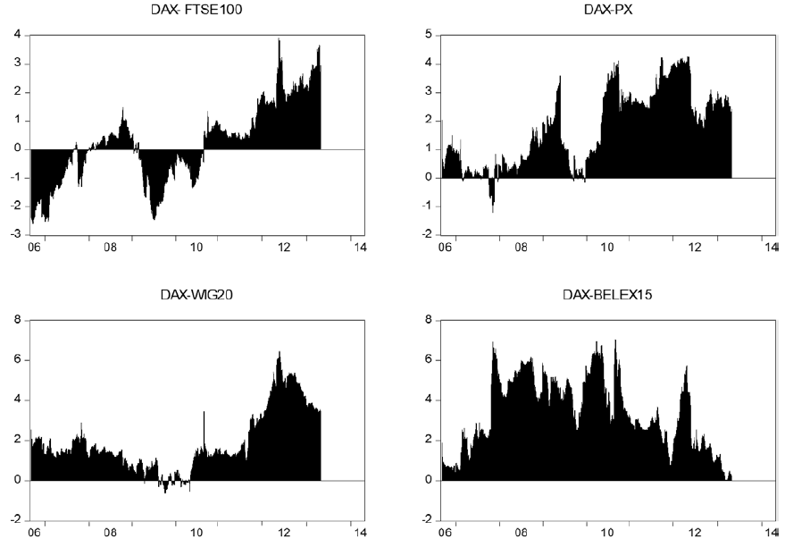
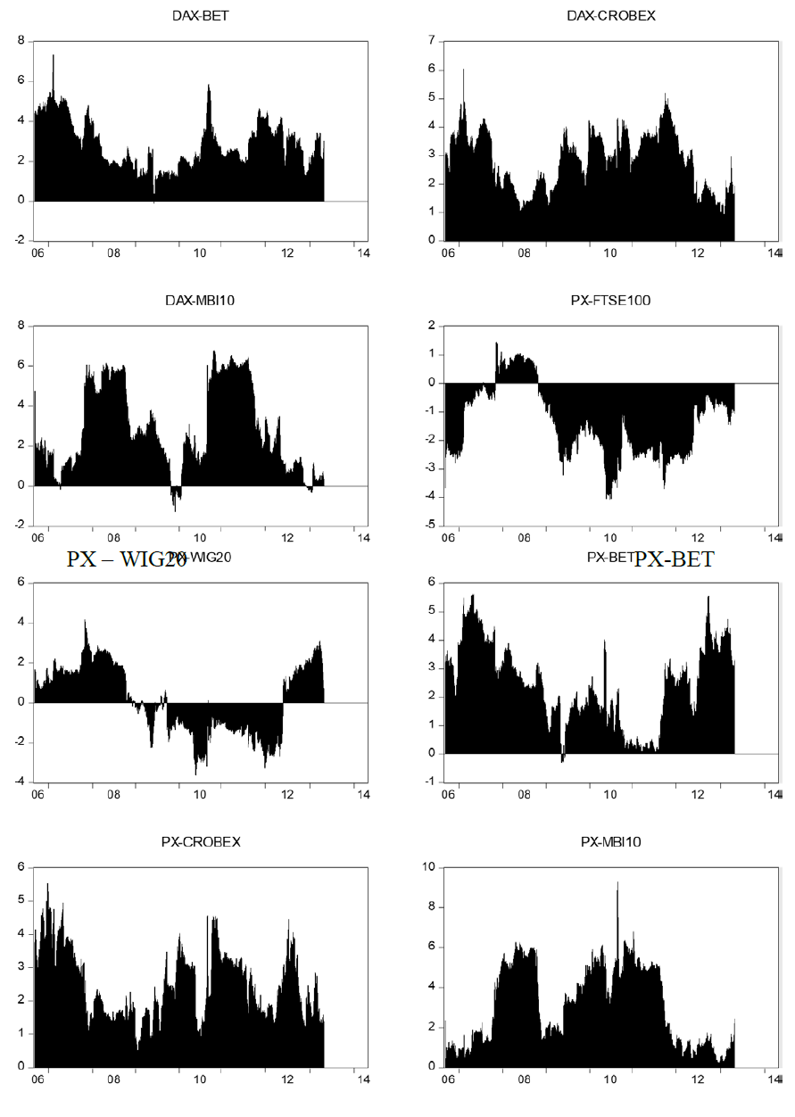
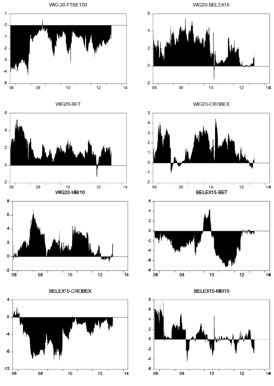
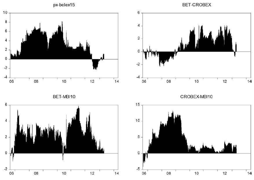
Net pairwise spillover indices are presented in the Figure 2. Positive values imply that the country i is a net transmitter to country j and negative values indicate that country i is a net receiver of spillovers. As expected, DAX and FTSE100 markets are net transmitters of spillovers to other markets. All of the analyzed markets are net receivers of spillovers from DAX and FTSE100, particularly during the periods of financial turmoil. There are bi-directional spillovers between DAX and FTSE100 indices. PX is a net transmitter of spillovers to BET, BELEX15, CROBEX and MBI10. Interestingly, the results indicate very high spillovers from the PX to Macedonian stock market (MBI10). Similarly to DAX and FTSE100, there are strong bi-directional spillovers between the PX and WIG20. WIG20 is a net transmitter of shocks to southeast European stock markets and to Romanian stock market. Serbian stock market (BELEX15) is a net receiver of spillovers from all other markets, except from MBI10. There is evidence of bi-directional spillover between Serbian and Macedonian stock market. Similarly to BELEX15, MBI10 is a net receiver of spillovers from the other stock markets. The results indicate strong spillovers from Croatian to Macedonian stock market.
Results from the VAR model:
• Total spillover index rise sharply during the periods of major financial and political events (US subprime mortgage crisis, Lehman Brothers collapse, Greek public debt revision, and the European Debt crisis) and remained at a high and stable level during the tranquil period.
• Net directional spillover index suggests that DAX and FTSE100 are the major net transmitters of spillover across other analyzed markets. On the other hand Southeast European markets (MBI10 and BELEX15) are net receivers of spillover from the other analyzed stock markets. However, there are relatively smaller effects of ’contagion’ from advanced markets to the Serbian and Macedonian stock markets relatively to their Central European counterparts. In the case of CROBEX and BET the spillover index from the other markets rapidly increases during the periods of financial disruptions (from 20-30% to almost 85%). In the case of Central European markets (PX and WIG20) spillover index varies from around 40-60% during the tranquil periods to almost 90% in the periods of financial disruptions. The results seem to be logical, indicating that MBI10 and BELEX15 are less integrated with the advanced financial markets. International investors can reduce their overall portfolio risk across Southeast stock markets.
• DAX and FTSE100 markets are net transmitters of spillovers to the other analyzed stock markets. There is bi-directional spillover between DAX and FTSE100, between PX and WIG-20 and between MBI10 and BELEX15.
In this part, we measure the volatility spillovers across the analyzed stock markets using the multivariate GARCH model. First, we estimate 8-variable multivariate BEKK-GARCH (1, 1) model. The stock market indices DAX, FTSE100, PX, WIG20, BELEX15, BET, CROBEX and MBI10 are noted 1, 2, 3, 4, 5, 6, 7 and 8 respectively. The results for the variance-covariance parameters are presented in the table 5. We will use different approach to model the return spillover, so here we only report the estimation results for the variance equation. The “A” terms (diagonal elements of matrix A) capture the own-shock (residual) spillovers (own ARCH effect). The B terms (diagonal B terms) capture the own volatility spillovers. Except DAX, FTSE100 and WIG20, own-lagged shocks on all other stock markets (A3,3; A5,5; A6,6; A7,7; A8,8) are statistically significant, which means that most of the markets exhibit own-shocks spillovers. Own-shocks spillovers are the highest for MBI10 (0,53) and for BET (0,42). The own-shocks spillover effects are smaller for the CROBEX, BELEX15 and PX indicating that own-shocks spillovers are less important for the more developed markets. Table 4 also reports statistically significant own-volatility spillovers in the case of PX, BELEX15, BET, CROBEX and MBI10. The results are in line with Li and Giles (2013), who found that advanced markets are less affected by their own past shocks and own past variances.
The results indicate several significant cross-volatility spillovers among the analyzed stock markets (off diagonal elements of matrix A and B). There is a positive unidirectional shocks spillover from DAX to CROBEX and from FTSE100 to WIG20. Also, there is a positive shock spillover from Czech stock market (PX) to Serbian and Romanian stock markets. Finally, there are positive unidirectional shock spillovers from WIG20 to PX, and from CROBEX to Macedonian stock market (MBI10). The results for the off-diagonal elements of matrix B indicate only one significant volatility spillover-from MBI10 to CROBEX.
GARCH BEKK estimation results | |||||||||
period 10/04/2005 to 03/27/2014 |
|
|
|
|
| ||||
| A | p-value | B | p-value |
| A | p-value | B | p-value |
(1,1) | 0.092 | 0.195 | 0.556 | 0.138 | (5,1) | 0.054 | 0.148 | 0.073 | 0.627 |
(1,2) | -0.031 | 0.638 | 0.042 | 0.904 | (5,2) | 0.066 | 0.044 | 0.059 | 0.676 |
(1,3) | 0.065 | 0.364 | -0.035 | 0.950 | (5,3) | 0.080 | 0.012 | -0.042 | 0.856 |
(1,4) | 0.019 | 0.830 | -0.024 | 0.963 | (5,4) | -0.006 | 0.867 | 0.051 | 0.804 |
(1,5) | 0.060 | 0.522 | 0.025 | 0.965 | (5,5) | 0.268 | 0.000 | 0.567 | 0.009 |
(1,6) | 0.025 | 0.652 | -0.082 | 0.786 | (5,6) | -0.036 | 0.143 | 0.014 | 0.917 |
(1,7) | 0.111 | 0.109 | -0.028 | 0.936 | (5,7) | 0.036 | 0.234 | 0.025 | 0.844 |
(1,8) | 0.024 | 0.732 | 0.037 | 0.927 | (5,8) | 0.027 | 0.396 | -0.137 | 0.334 |
(2,1) | 0.042 | 0.578 | -0.114 | 0.793 | (6,1) | 0.039 | 0.430 | 0.055 | 0.425 |
(2,2) | 0.089 | 0.186 | 0.424 | 0.246 | (6,2) | 0.088 | 0.037 | 0.007 | 0.908 |
(2,3) | 0.051 | 0.499 | -0.067 | 0.892 | (6,3) | 0.164 | 0.000 | 0.027 | 0.756 |
(2,4) | 0.217 | 0.022 | -0.353 | 0.489 | (6,4) | 0.027 | 0.663 | 0.099 | 0.255 |
(2,5) | 0.060 | 0.576 | -0.156 | 0.757 | (6,5) | 0.127 | 0.004 | 0.021 | 0.793 |
(2,6) | 0.084 | 0.180 | -0.026 | 0.939 | (6,6) | 0.427 | 0.000 | 0.789 | 0.000 |
(2,7) | -0.009 | 0.912 | -0.090 | 0.825 | (6,7) | -0.013 | 0.757 | -0.076 | 0.188 |
(2,8) | 0.055 | 0.437 | -0.093 | 0.817 | (6,8) | 0.002 | 0.955 | 0.079 | 0.201 |
(3,1) | 0.024 | 0.625 | 0.007 | 0.957 | (7,1) | 0.022 | 0.514 | 0.006 | 0.846 |
(3,2) | 0.032 | 0.433 | 0.011 | 0.926 | (7,2) | 0.032 | 0.294 | 0.014 | 0.613 |
(3,3) | 0.238 | 0.000 | 0.273 | 0.071 | (7,3) | 0.045 | 0.232 | -0.023 | 0.612 |
(3,4) | 0.041 | 0.444 | 0.048 | 0.765 | (7,4) | 0.009 | 0.828 | 0.010 | 0.811 |
(3,5) | 0.128 | 0.017 | 0.028 | 0.872 | (7,5) | -0.025 | 0.462 | -0.004 | 0.905 |
(3,6) | 0.063 | 0.055 | -0.026 | 0.839 | (7,6) | 0.001 | 0.942 | -0.001 | 0.971 |
(3,7) | -0.003 | 0.926 | 0.032 | 0.828 | (7,7) | 0.279 | 0.000 | 0.941 | 0.000 |
(3,8) | -0.039 | 0.304 | 0.036 | 0.821 | (7,8) | 0.068 | 0.005 | -0.007 | 0.707 |
(4,1) | -0.041 | 0.335 | -0.007 | 0.979 | (8,1) | 0.045 | 0.224 | 0.015 | 0.656 |
(4,2) | -0.042 | 0.274 | -0.099 | 0.642 | (8,2) | 0.049 | 0.105 | 0.014 | 0.697 |
(4,3) | 0.065 | 0.092 | -0.151 | 0.603 | (8,3) | 0.014 | 0.722 | 0.038 | 0.483 |
(4,4) | -0.002 | 0.960 | 0.445 | 0.141 | (8,4) | -0.007 | 0.868 | 0.045 | 0.368 |
(4,5) | 0.046 | 0.311 | -0.084 | 0.794 | (8,5) | 0.017 | 0.625 | 0.014 | 0.742 |
(4,6) | 0.002 | 0.958 | -0.035 | 0.861 | (8,6) | 0.045 | 0.050 | 0.025 | 0.313 |
(4,7) | 0.038 | 0.272 | -0.074 | 0.752 | (8,7) | -0.011 | 0.703 | 0.047 | 0.019 |
(4,8) | 0.056 | 0.103 | -0.025 | 0.923 | (8,8) | 0.534 | 0.000 | 0.840 | 0.000 |
However, it is very hard for the estimated GARCH BEKK model to be interpreted in the economic sense (Li and Majerowska, 2006). To overcome this issue, we create conditional correlation plots based on estimated model. The time-varying conditional correlation plots are presented in Figure 3. The results suggest a strong connection between Central European market (PX and WIG20) and their western counterparts (DAX and FTSE100). The conditional correlation coefficient between DAX and PX and between DAX and WIG20 varies from 0,80 and 0,65 during the tranquil periods to almost 0,9 during the periods of financial turmoil (for PX and WIG 20 respectively). There is only a modest connection between Croatian and Romanian market and Western markets. The correlation varies around 40% most of the time, while in the period of financial crisis correlation coefficient rises sharply. There is no evidence of connection between Macedonian and Serbian stock markets and the advanced western markets. The correlation coefficient varies around zero for most of the time. However, during the period of the financial crisis, correlation coefficient rose to almost 0,5 suggesting some evidence of volatility spillovers from the advanced markets during the period of financial crisis.


6. Conclusion
This paper analyzed the return spillovers, volatility spillovers and stock market co-movements among Western, Central and Southeast European stock markets. Following Diebold and Yilmaz (2012), we created the spillover index based on a generalized VAR framework. The “total spillover index” rose sharply during the periods of major financial and political events (US subprime mortgage crisis, Lehman Brothers collapse, Greek public debt revision, and the European Debt crisis) and remained at a high and stable level during the tranquil periods.
The results show that Western markets are the biggest net transmitters of spillover to Central and Southeast European markets. On the other side, in the terms of “return spillovers”, Serbian and Macedonian markets are the biggest net receivers of spillover from the other six markets. There are relatively small effects of “contagion” from the advanced markets to Serbian and Macedonian stock markets relatively to their Central European counterparts. In the case of CROBEX and BET the spillover index from the other markets rapidly increases during the periods of financial disruptions (from 20-30% to almost 85%). In the case of Central European markets (PX and WIG20) spillover index varies from around 40-60% during the tranquil periods to almost 90% in the periods of financial disruptions. The results seem to be logical, indicating that MBI10 and BELEX15 are less integrated with the advanced financial markets. International investors can reduce their overall portfolio risk across Southeast stock markets. During the financial crisis of 2007, most of the spillovers to the Macedonian and Serbian stock market came from Croatian, German and Czech stock market. During the European debt crisis, most of the spillovers to the Serbian and Macedonian markets came from German, Czech and Romanian market. There are bi-directional spillovers between DAX and FTSE100, PX and WIG20 and between MBI10 and BELEX15. Unlike the Southeast market, the spillovers to the PX and WIG20 came mostly from DAX and FTSE100.
The volatility spillovers and stock market co-movements were analyzed with the multivariate GARCH BEKK (1,1) model. The results indicate several significant cross-volatility spillovers among the analyzed stock markets (off diagonal elements of matrix A and B). There are positive unidirectional shock spillovers from DAX to CROBEX and from FTSE100 to WIG20. Also, there is a positive shock spillover from Czech stock market (PX) to Serbian and Romanian stock markets. Finally, there are positive unidirectional shock spillovers from WIG20 to PX, and from CROBEX to Macedonian stock market (MBI10). The results for the off-diagonal elements of matrix B indicate only one significant volatility spillover-from MBI10 to CROBEX. Because it is hard to analyze the estimated coefficients from the GARCH BEKK model, we estimated the time-varying conditional correlation coefficients. The results suggest a strong connection between Central European market (PX and WIG20) and their western counterparts (DAX and FTSE100). The conditional correlation coefficient between DAX and PX and between DAX and WIG20 varies from 0,80 and 0,65 during the tranquil periods to almost 0,9 during the periods of financial turmoil (for PX and WIG 20 respectively). There is only a modest connection between Croatian and Romanian markets and Western markets. The correlation varies around 0,4 most of the time, while in the period of financial crisis correlation coefficient rises sharply. There is no evidence of a connection between Macedonian and Serbian stock markets and the advanced western markets. The correlation coefficient varies around zero for most of the time. However, during the period of the financial crisis, correlation coefficient rose to almost 0,5 suggesting some evidence of volatility spillovers from the advanced markets during the period of financial crisis.
The data used to support the findings of this study are available from the corresponding author upon request.
The authors declare that they have no conflicts of interest.
Figure 1. Log-Index values on eight stock markets (04/10/2005- 03/03/2014)
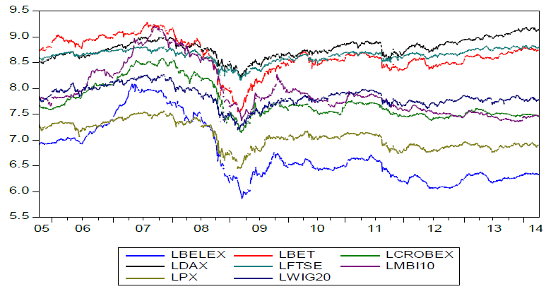
Figure 2. Daily Return Series
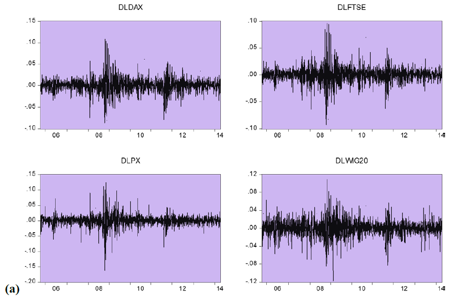
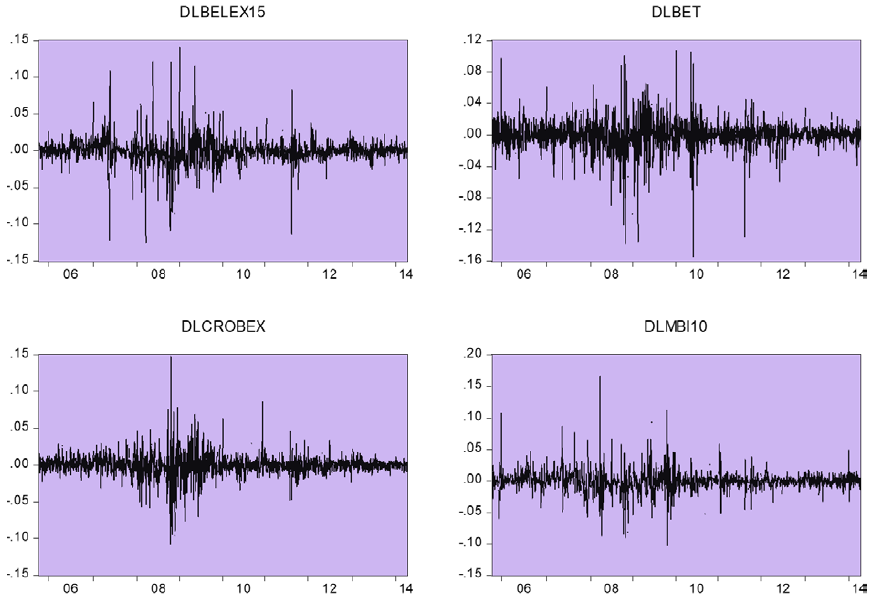
Figure 5. Net pairwise spillover indices
